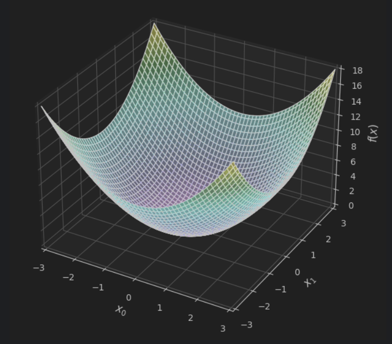
一个二元函数的图像
import numpy as np
import matplotlib.pyplot as plt

# 生成数据
x0 = np.linspace(-3, 3, 100)
x1 = np.linspace(-3, 3, 100)
X0, X1 = np.meshgrid(x0, x1)
Z = X0**2 + X1**2

# 创建3D画布
fig = plt.figure(figsize=(10, 7))
ax = fig.add_subplot(111, projection='3d')

# 绘制曲面
surf = ax.plot_surface(X0, X1, Z,
                      cmap='viridis',  # 颜色映射
                      edgecolor='k',   # 网格线颜色
                      alpha=0.8)       # 透明度
#
# 坐标轴设置
ax.set_xlabel('$x_0$', fontsize=12)
ax.set_ylabel('$x_1$', fontsize=12)
ax.set_zlabel('$f(x)$', fontsize=12)
ax.set_xlim(-3, 3)
ax.set_ylim(-3, 3)
ax.set_zlim(0, 18)

# 添加颜色条
# fig.colorbar(surf, shrink=0.5, aspect=5)

# 视角调整(可选)
# ax.view_init(elev=30, azim=45)  # 仰角30度,方位角45度

plt.show()
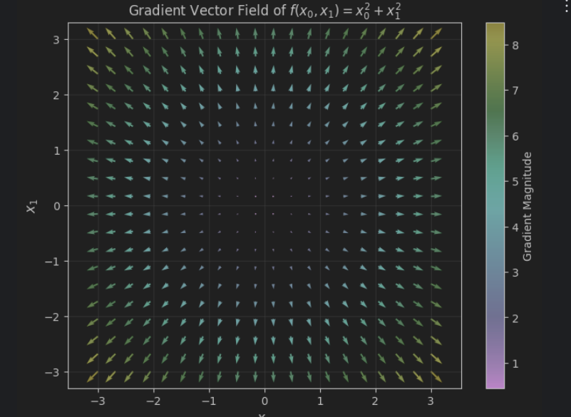
该函数的梯度图像
import numpy as np
import matplotlib.pyplot as plt

# 生成网格数据
x0 = np.linspace(-3, 3, 20)  # 减少点数避免箭头过密
x1 = np.linspace(-3, 3, 20)
X0, X1 = np.meshgrid(x0, x1)

# 计算梯度(手动求导)
df_dx0 = 2 * X0  # 对x0的偏导数
df_dx1 = 2 * X1  # 对x1的偏导数

# 计算梯度幅值(箭头颜色)
grad_magnitude = np.sqrt(df_dx0**2 + df_dx1**2)

# 创建画布
plt.figure(figsize=(8, 6))

# 绘制梯度向量场
quiver = plt.quiver(X0, X1, df_dx0, df_dx1, grad_magnitude,
                   cmap='viridis',      # 颜色映射
                   angles='xy',        # 箭头方向基于xy坐标系
                   scale_units='xy',   # 缩放单位一致
                   scale=30,           # 箭头缩放比例(值越小箭头越大)
                   width=0.004,        # 箭头宽度
                   headwidth=3)        # 箭头头部宽度

# 添加颜色条
plt.colorbar(quiver, label='Gradient Magnitude')

# 图形装饰
plt.title('Gradient Vector Field of $f(x_0, x_1) = x_0^2 + x_1^2$', fontsize=12)
plt.xlabel('$x_0$', fontsize=12)
plt.ylabel('$x_1$', fontsize=12)
plt.grid(alpha=0.3)
plt.axis('equal')  # 保持坐标轴比例一致

plt.show()
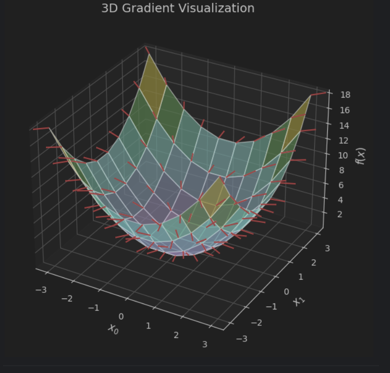
三维的梯度图像
import numpy as np
import matplotlib.pyplot as plt
from mpl_toolkits.mplot3d import Axes3D

# 生成数据
x0 = np.linspace(-3, 3, 10)  # 稀疏网格避免箭头拥挤
x1 = np.linspace(-3, 3, 10)
X0, X1 = np.meshgrid(x0, x1)
Z = X0**2 + X1**2

# 计算梯度
df_dx0 = 2 * X0
df_dx1 = 2 * X1
df_dz = np.ones_like(Z)  # 梯度在z方向的分量(投影到三维空间)

# 创建3D画布
fig = plt.figure(figsize=(10, 7))
ax = fig.add_subplot(111, projection='3d')

# 绘制抛物面
ax.plot_surface(X0, X1, Z,
                cmap='viridis',
                alpha=0.7,
                edgecolor='k')

# 绘制三维梯度箭头
ax.quiver(X0, X1, Z,         # 箭头起点
          df_dx0, df_dx1, df_dz,  # 箭头分量
          length=0.5,        # 箭头长度
          color='red',        # 箭头颜色
          normalize=True,    # 归一化箭头长度(统一显示方向)
          arrow_length_ratio=0.03)  # 箭头头部比例

# 坐标轴设置
ax.set_xlabel('$x_0$', fontsize=12)
ax.set_ylabel('$x_1$', fontsize=12)
ax.set_zlabel('$f(x)$', fontsize=12)
ax.set_title('3D Gradient Visualization', fontsize=14)

plt.show()
梯度下降法的实现
def numerical_gradient(f, x):
    h = 1e-4
    grad = np.zeros_like(x)

    for idx in range(x.size):
        tmp_val = x[idx]
        x[idx]=tmp_val + h
        fxh1 = f(x)

        x[idx] = tmp_val -h
        fxh2 = f(x)

        grad[idx]=(fxh1 - fxh2) / (2*h)
        x[idx] = tmp_val
    return grad


def gradient_descend(f,init_x,lr =0.01,step_num=100):
    x = init_x

    for i in range(step_num):
        grad = numerical_gradient(f,x)
        x -= lr * grad

    return x

def f(x):
    return x[0]**2 + x[1]**2

init_x = np.array([-3.0,4.0])
gradient_descend(f,init_x,lr=0.1,step_num=100)
梯度更新过程
import numpy as np
import matplotlib.pyplot as plt
# 定义目标函数和梯度
def f(x0, x1):
    return x0**2 + x1**2

def gradient(x0, x1):
    return np.array([2*x0, 2*x1])  # 梯度向量

# 梯度下降参数
initial_point = np.array([-3.0, 4.0])  # 初始位置
learning_rate = 0.1                    # 学习率
max_iterations = 20                     # 最大迭代次数
tolerance = 1e-6                        # 收敛阈值

# 生成等高线数据
x0 = np.linspace(-4, 4, 100)
x1 = np.linspace(-5, 5, 100)
X0, X1 = np.meshgrid(x0, x1)
Z = f(X0, X1)

# 运行梯度下降
path = [initial_point.copy()]
current_point = initial_point.copy()

for _ in range(max_iterations):
    grad = gradient(*current_point)
    if np.linalg.norm(grad) < tolerance:
        break
    current_point -= learning_rate * grad
    path.append(current_point.copy())

path = np.array(path)

# 可视化设置
plt.figure(figsize=(10, 6))

# 绘制等高线
contour = plt.contour(X0, X1, Z,
                     levels=np.logspace(0, 2, 10),  # 指数间隔的等高线
                     cmap='gray',
                     linestyles='--',
                     linewidths=0.5)
plt.clabel(contour, inline=True, fontsize=8)  # 添加等高线数值标签

# 绘制梯度下降路径
plt.plot(path[:,0], path[:,1],
        'o-',                  # 圆形标记+实线
        color='#FF6347',       # 番茄红色
        markersize=8,
        linewidth=2,
        markeredgecolor='black',
        label='Gradient Descent Path')

# 添加路径箭头
for i in range(1, len(path)):
    dx = path[i,0] - path[i-1,0]
    dy = path[i,1] - path[i-1,1]
    plt.arrow(path[i-1,0], path[i-1,1], dx*0.8, dy*0.8,  # 缩短箭头避免重叠
              shape='full',
              color='dodgerblue',
              width=0.02,
              head_width=0.3)

# 标注特殊点
plt.scatter(*initial_point, s=150, zorder=3,
           marker='*',
           color='gold',
           edgecolor='black',
           label='Start (-3, 4)')
plt.scatter(0, 0, s=100,
           marker='X',
           color='limegreen',
           edgecolor='black',
           label='Minimum (0, 0)')

# 图形装饰
plt.title("Gradient Descent on $f(x_0, x_1) = x_0^2 + x_1^2$", fontsize=14)
plt.xlabel('$x_0$', fontsize=12)
plt.ylabel('$x_1$', fontsize=12)
plt.xlim(-3.5, 1)
plt.ylim(-1, 4.5)
plt.grid(alpha=0.3)
plt.legend(loc='upper right')
plt.gca().set_aspect('equal')  # 保持坐标轴比例一致

plt.show()
SGD 随机梯度下降法
from torch import sigmoid, softmax
import sys, os
sys.path.append(os.pardir)
from common.functions import *
from common.gradient import numerical_gradient
class TwoLayerNet:
    def __init__(self, input_size, hidden_size, output_size,
    weight_init_std=0.01):
 # 初始化权重
         self.params = {}
         self.params['W1'] = weight_init_std * \
         np.random.randn(input_size, hidden_size)
         self.params['b1'] = np.zeros(hidden_size)
         self.params['W2'] = weight_init_std * \
         np.random.randn(hidden_size, output_size)
         self.params['b2'] = np.zeros(output_size)
     def predict(self, x):
         W1, W2 = self.params['W1'], self.params['W2']
         b1, b2 = self.params['b1'], self.params['b2']
         a1 = np.dot(x, W1) + b1
         z1 = sigmoid(a1)
         a2 = np.dot(z1, W2) + b2
         y = softmax(a2)
         return y
     # x:输入数据, t:监督数据
     def loss(self, x, t):
         y = self.predict(x)
         return cross_entropy_error(y, t)
     def accuracy(self, x, t):
         y = self.predict(x)
         y = np.argmax(y, axis=1)
         t = np.argmax(t, axis=1)
         accuracy = np.sum(y == t) / float(x.shape[0])
         return accuracy
     # x:输入数据, t:监督数据
     def numerical_gradient(self, x, t):
         loss_W = lambda W: self.loss(x, t)
         grads = {}
         grads['W1'] = (numerical_gradient(loss_W, self.params['W1']))
         grads['b1'] = numerical_gradient(loss_W, self.params['b1'])
         grads['W2'] = numerical_gradient(loss_W, self.params['W2'])
         grads['b2'] = numerical_gradient(loss_W, self.params['b2'])
         return grads

 浙公网安备 33010602011771号