Pointnet++论文学习
背景
在PointNet中并没有局部特征的概念,要么是对单个物体进行处理获取单个特征,要么是进行整体最大池化获取全局特征,丢失了很多局部信息。也是因此在进行分割物体时效果显得一般,Pointnet++则优化了这个问题。
方法
Pointnet++在Point的基础上增添了多层次结构,使得网络能够在越来越大的区域上提供更高级别的特征,这个提取过程称为Set abstraction,主要包含三个部分,Sampling layer, Grouping layer以及 PointNet layer,如下图所示

接下来进行分层介绍:
Sampling layer
使用farthest point sampling(FPS)选择 N 个点,作者使用FPS而不是随机取样的原因是,FPS更容易包含整个点云。那么什么是FPS呢,我们这里进行简单介绍。FPS算法我们可以简单理解为以下几步:
1、随机设定一个点x作为我们选中的集合S里的第一点
2、计算其他点离这个点的距离,从中选出距离最远的x1作为第二点,加入集合,此时的S={x,x1}
3、计算其他点离这两个点的距离,比如存在点X2,我们就要计算|X2-X|与|x2-X1|,然后从中选出距离最近的作为它离集合的距离
4、计算与集合之中的距离,不断迭代,直至集合S满足我们设定的阈值K
FPS算法的核心目标是是从一个大的点集中,选取一个有代表性的、在空间上分布均匀的子集,所以它每次都选取距离当前已选点集最远的那个点补充到集合中,这样就可以实现分布均匀,有代表性。
这里通过FPS来抽样点集中较为重要的点(即任务是找到点云集中的局部区域的中心点)。
grouping layer
这里的主要目的是从每个点中,我们要找出它对应的局部邻域,以便后续的算法能够在这个邻域中提取局部特征。
这里采用Ball Query和KNN都是可以的(在本文中采用的是Ball Query),这里再对这两个算法进行介绍。
Ball Query是指的球查询,具体如下
1、我们设定一组中心点,然后选定半径R,再设定邻居数量K,接下来输入就已经完成
2、我们对于每一个中心点,计算其离点云中的其他点的距离,然后距离从小到大挑选出前K个,作为邻域点。
K-Nearest Neighbors,即K近邻,他的核心思想是以固定的邻居数量来定义邻域。 对于每个中心点,无论远近,只找离它最近的K个点。
其具体方法如下所示:
1、在整个点云P设定一组中心点,设定邻居数量K。
2、对于每一个中心点,我们计算中心点到点云中其他点的距离,将这些点按照距离从小到大排序。
3、选取前K个点,这K个点就是中心点的邻域。
这两个方法都可以为每个中心点定义局部邻域,以便进行局部特征聚合(在本文中使用PointNet进行),当分布不太均匀时,Ball Query就更适合,而在均匀时KNN则更为适合。
总之,Grouping layer的任务是通过中心点找到邻居点,并将它们组织称为局部区域集。
PointNet layer
将局部区域中的点使用Pointnet进行处理,通过共享MLP和对称聚合函数,将任意数量的无序局部点云编码为一个固定长度的、具有判别力的特征向量。利用相对坐标与点特征相结合的方式可以捕获局部区域中点与点之间的关系。
MSG && MRG
不同于图片数据分布在规则的像素网格上且有均匀的数据密度,点云数据在空间中的分布是不规则且不均匀的。当点云不均匀时,每个子区域中如果在分区的时候使用相同的球半径,会导致部分稀疏区域采样点过小。作者提出多尺度成组 (MSG)和多分辨率成组 (MRG)两种解决办法。
MSG的核心思想 :对同一个中心点,同时使用多个不同尺度(半径) 来构建邻域,提取不同尺度的特征,然后将这些特征拼接起来。
具体的工作方式是
1、对于同一个关键点,使用一组不同的半径 [r1, r2, r3, ...] 和不同的邻域点数 [n1, n2, n3, ...],分别执行 sample_and_group 操作。
2、每个尺度分组得到的局部点集,都独立地通过一个 PointNet 层,为该尺度提取一个特征向量。
3、将所有不同尺度提取出的特征向量拼接 在一起,形成该关键点的最终多尺度特征。
它的优点是性能好,鲁棒性强,但缺点也显而易见,计算和内存开销巨大。
MRG的核心思想是利用上一层已经计算好的特征。

具体的工作方式是:
1、在输入点云中使用单一尺度进行sample_and_group操作,获取了高分辨率的局部几何细节。
2、取出上一层的特征,由于上一层是下采样后的点云,其每个点本身就代表了更大范围的区域(拥有更大的感受野),因此这个特征已经包含了低分辨率的更广泛的上下文信息。
3、将两者进行拼接,实现全局+局部的信息。
代码实现
Sampling && grouping layer
这里是使用的sample_and_group函数,它的作用将之前所说的前两个层进行融合,即进行采样关键点,再为每个关键点建立局部邻域,提取这些局部区域中的点及其特征
def sample_and_group(npoint, radius, nsample, xyz, points, returnfps=False):
    """
    Input:
        npoint: 采样的关键点数量
        radius: 构建局部邻域的半径
        nsample: 每个邻域内采样的关键点数量
        xyz: 点云坐标数据 , [B, N, 3],B是批量大小,N是点的数量,3是坐标维度
        points: 点的特征数据(可选), [B, N, D],D是通道数
    Return:
        new_xyz: 采样得到的关键点坐标, [B, npoint, nsample, 3]
        new_points: 每个关键点对应的局部区域点和特征, [B, npoint, nsample, 3+D]
    """
    B, N, C = xyz.shape
    S = npoint
    # 使用 最远点采样(FPS) 从原始点云中选出 npoint 个具有代表性的点。
    fps_idx = farthest_point_sample(xyz, npoint) # [B, npoint]
    new_xyz = index_points(xyz, fps_idx) # [B, npoint, 3]
    # 对于每个选中的关键点,使用 球查询(Ball Query) 找出它周围距离小于 radius 的所有邻近点。
    # 最多保留 nsample 个点,如果不够就重复最近的点来填充。
    idx = query_ball_point(radius, nsample, xyz, new_xyz)
    # 把刚才找到的邻近点的坐标提取出来。
    grouped_xyz = index_points(xyz, idx) # [B, npoint, nsample, 3]
    # 把它们相对于关键点的位置进行归一化(平移中心到以关键点为原点的局部坐标系上)。
    grouped_xyz_norm = grouped_xyz - new_xyz.view(B, S, 1, C) # [B, npoint, nsample, 3]

    # 如果有额外的点特征(比如颜色、法线等),也一并提取。
    if points is not None:
        grouped_points = index_points(points, idx)
        # 把邻近点的坐标和特征拼接在一起,形成最终的局部区域表示。
        new_points = torch.cat([grouped_xyz_norm, grouped_points], dim=-1) # [B, npoint, nsample, C+D]
    else:
        new_points = grouped_xyz_norm

    if returnfps:
        return new_xyz, new_points, grouped_xyz, fps_idx
    else:
        return new_xyz, new_points
这里再看一下farthest_point_sample函数和index_points的具体实现
def farthest_point_sample(xyz, npoint):
    """
    Input:
        xyz: pointcloud data, [B, N, 3] ,同之前,B是批量大小,N是点数,3是三维
        npoint: number of samples,即关键点的数量
    Return:
        centroids: sampled pointcloud index, [B, npoint]
    """
    device = xyz.device
    B, N, C = xyz.shape
    #初始化结果容器,centroids 形状为 [B, npoint],用于存储每个批次中每个采样点的索引。
    centroids = torch.zeros(B, npoint, dtype=torch.long).to(device)
    #初始化距离矩阵:distance 形状为 [B, N],记录每个点到已选点集的最小距离。
    distance = torch.ones(B, N).to(device) * 1e10
    #随机选择第一个点:farthest 形状为 [B],存储每个批次当前轮次选中的点索引。
    farthest = torch.randint(0, N, (B,), dtype=torch.long).to(device)
    #创建批次索引:[0, 1, 2, ..., B-1],用于后续的批次索引操作。
    batch_indices = torch.arange(B, dtype=torch.long).to(device)
    for i in range(npoint):
        #记录当前选中的点:将本轮选中的点索引 farthest 存入结果矩阵的第 i 列
        centroids[:, i] = farthest
        #获取每个批次当前选中点的坐标,同时使用view多增加一个维度,为广播做准备
        centroid = xyz[batch_indices, farthest, :].view(B, 1, 3)
        #计算所有点到当前选中点的距离
        dist = torch.sum((xyz - centroid) ** 2, -1)
        #计算距离比之前的中心点集合小的
        mask = dist < distance
        #覆盖
        distance[mask] = dist[mask]
        #沿着最后一个维度(点的维度)求最大值,取出第二个元素,即最大值的索引
        farthest = torch.max(distance, -1)[1]
    return centroids
farthest_point_sample的函数其实就是FPS算法的代码实现,找到前K个中心点。
接下来我们看index_points函数,它的作用是使用批次索引矩阵和点索引矩阵,从批量点云数据中精确地采集指定的点,保持输出形状与索引矩阵一致,简单说就是聚合点
def index_points(points, idx):
    """
    Input:
        points: input points data, [B, N, C]
        idx: sample index data, [B, S]
    Return:
        new_points:, indexed points data, [B, S, C]
    """
    device = points.device
    B = points.shape[0]#获取批量大小
    view_shape = list(idx.shape)#获取{B,S}
    view_shape[1:] = [1] * (len(view_shape) - 1)#将1之后的其他维度全部填充为1,这里其实就是由[B,S]-->[B,1]
    repeat_shape = list(idx.shape)
    repeat_shape[0] = 1#[B,S]-->[1,S]
    #创建[0,1,....,B-1],重塑为[B,1],再重塑为[B,S]
    batch_indices = torch.arange(B, dtype=torch.long).to(device).view(view_shape).repeat(repeat_shape)
    #执行索引采集
    new_points = points[batch_indices, idx, :]
    return new_points
接下来是球查询query_ball_point的实现
def query_ball_point(radius, nsample, xyz, new_xyz):
    """
    Input:
        radius: local region radius
        nsample: max sample number in local region
        xyz: all points, [B, N, 3]
        new_xyz: query points, [B, S, 3]
    Return:
        group_idx: grouped points index, [B, S, nsample]
    """
    device = xyz.device
    B, N, C = xyz.shape
    _, S, _ = new_xyz.shape # 查询点数量(比如通过 FPS 得到的质心)
    # 构造一个从 0 到 N-1 的索引数组,代表原始点云中每个点的“身份证号”
    # 然后复制这个索引数组到每个 batch 和每个查询点上,形成 [B, S, N] 的结构
    group_idx = torch.arange(N, dtype=torch.long).to(device).view(1, 1, N).repeat([B, S, 1])
    # 计算每个查询点(new_xyz)与原始点(xyz)之间的平方欧氏距离
    # 输出形状为 [B, S, N]:每个查询点对所有原始点的距离
    sqrdists = square_distance(new_xyz, xyz)
    # 把距离超过 radius^2 的点全部替换为 N(一个非法索引),表示“这些人离我太远了,我不感兴趣。”
    group_idx[sqrdists > radius ** 2] = N
    # 对每个查询点的邻近点按索引排序(因为前面有 N,所以小的才是有效点)
    # 然后只保留前 nsample 个点
    group_idx = group_idx.sort(dim=-1)[0][:, :, :nsample]
    # 如果某个查询点附近的点太少,有些位置被标记为 N(无效)。
    # 我们就用该查询点最近的那个点(第一个点)去填充这些空缺。
    group_first = group_idx[:, :, 0].view(B, S, 1).repeat([1, 1, nsample])
    mask = group_idx == N
    group_idx[mask] = group_first[mask]
    return group_idx # (batch,npoint,nsample)
sample_and_group_all函数将整个点云视为一个大局部区域,对所有点进行特征提取,如果有额外特征则进行合并。
def sample_and_group_all(xyz, points):
    """
    Input:
        xyz: input points position data, [B, N, 3], 点云坐标数据
        points: input points data, [B, N, D], 点云的额外特征(如法线、颜色等)
    Return:
        new_xyz: sampled points position data, [B, 1, 3]
        new_points: sampled points data, [B, 1, N, 3+D]
    """
    device = xyz.device
    B, N, C = xyz.shape
    # 创建一个全零点作为“质心”
    # 虽然这个点没有实际意义,但它是为了统一接口设计的一个占位符
    new_xyz = torch.zeros(B, 1, C).to(device)
    # 把原始点云 reshape 成一个大的局部区域
    grouped_xyz = xyz.view(B, 1, N, C)
    # 如果有额外特征(比如法线、颜色),也一并加入
    if points is not None:
        # 终输出的 new_points 是 [B, 1, N, 3+D],代表每个 batch 中只有一组“大区域”的点及其特征
        new_points = torch.cat([grouped_xyz, points.view(B, 1, N, -1)], dim=-1)
    else:
        new_points = grouped_xyz
    return new_xyz, new_points # 全局质心点(0 位置), 所有点组成的局部区域
接下来就是PointNetSetAbstraction,它是Pointnet++的核心模块,它的作用是负责从输入的点云数据中采样关键点,构建它们的局部邻域区域,并通过一个小型 PointNet 提取这些区域的高维特征,从而实现点云的分层特征学习。
class PointNetSetAbstraction(nn.Module):
    def __init__(self, npoint, radius, nsample, in_channel, mlp, group_all):
        super(PointNetSetAbstraction, self).__init__()
        self.npoint = npoint # 采样的关键点数量
        self.radius = radius # 构建局部邻域的半径
        self.nsample = nsample # 每个邻域内采样的关键点数量
        self.mlp_convs = nn.ModuleList()
        self.mlp_bns = nn.ModuleList()
        last_channel = in_channel # 输入点的特征维度
        for out_channel in mlp:
            self.mlp_convs.append(nn.Conv2d(last_channel, out_channel, 1))
            self.mlp_bns.append(nn.BatchNorm2d(out_channel))
            last_channel = out_channel
        self.group_all = group_all

    def forward(self, xyz, points):
        """
        Input:
            xyz: input points position data, [B, C, N]
            points: input points data, [B, D, N]
        Return:
            new_xyz: sampled points position data, [B, C, S]
            new_points_concat: sample points feature data, [B, D', S]
        """
        xyz = xyz.permute(0, 2, 1) # [B, N, C]
        if points is not None:
            points = points.permute(0, 2, 1)

        # 如果 group_all=True,则对整个点云做全局特征提取。
        if self.group_all:
            new_xyz, new_points = sample_and_group_all(xyz, points)
        else:
        # 否则使用 FPS(最远点采样)选关键点,再用 Ball Query 找出每个点的局部邻近点。
            # 参数: 质点数量,采样半径,采样点数量,点坐标,点额外特征
            new_xyz, new_points = sample_and_group(self.npoint, self.radius, self.nsample, xyz, points)
        # 局部特征编码(Mini-PointNet)
        # new_xyz: sampled points position data, [B, npoint, C]
        # new_points: sampled points data, [B, npoint, nsample, C+D]
        # 把邻域点的数据整理成适合卷积的格式 [B, C+D, nsample, npoint]
        new_points = new_points.permute(0, 3, 2, 1)
        # 使用多个 Conv2d + BatchNorm + ReLU 层提取特征
        for i, conv in enumerate(self.mlp_convs):
            bn = self.mlp_bns[i]
            new_points =  F.relu(bn(conv(new_points))) # [B, out_channel , nsample, npoint]

        # 对每个局部区域内所有点的最大响应值进行池化,得到该区域的固定长度特征表示。
        # 在 new_points 的第 2 个维度(即每个局部邻域内的点数量维度)上做最大池化(max pooling)。
        # 输出形状为 [B, out_channel, npoint],即每个查询点有一个特征向量。
        new_points = torch.max(new_points, 2)[0] # [B, out_channel, npoint]
        new_xyz = new_xyz.permute(0, 2, 1) # [B, C, npoint]
        return new_xyz, new_points # 查询点的位置(质心) , 每个查询点点局部特征。
分类
单尺度分组分类模型
这里使用单尺度的分组分类,使用多层SetAbstracttion提取点云的层次化特征,最终输出分类结果
# pointnet2_cls_ssg.py
class get_model(nn.Module):
   # num_class: 输出类别数
   # normal_channel: 是否包含法线信息(默认有 (x,y,z,nx,ny,nz),否则只有 (x,y,z))
   def __init__(self,num_class,normal_channel=True):
       super(get_model, self).__init__()
       in_channel = 6 if normal_channel else 3
       self.normal_channel = normal_channel
       # PointNet++ 的核心就是逐层提取局部特征。这里的三个 SA 层构成了一个 三层分层特征学习结构 :
       self.sa1 = PointNetSetAbstraction(npoint=512, radius=0.2, nsample=32, in_channel=in_channel, mlp=[64, 64, 128], group_all=False)
       self.sa2 = PointNetSetAbstraction(npoint=128, radius=0.4, nsample=64, in_channel=128 + 3, mlp=[128, 128, 256], group_all=False)
       self.sa3 = PointNetSetAbstraction(npoint=None, radius=None, nsample=None, in_channel=256 + 3, mlp=[256, 512, 1024], group_all=True)
       self.fc1 = nn.Linear(1024, 512)
       self.bn1 = nn.BatchNorm1d(512)
       self.drop1 = nn.Dropout(0.4)
       self.fc2 = nn.Linear(512, 256)
       self.bn2 = nn.BatchNorm1d(256)
       self.drop2 = nn.Dropout(0.4)
       self.fc3 = nn.Linear(256, num_class)

   def forward(self, xyz):
       B, _, _ = xyz.shape
       if self.normal_channel:
           norm = xyz[:, 3:, :]
           xyz = xyz[:, :3, :]
       else:
           norm = None
       l1_xyz, l1_points = self.sa1(xyz, norm)
       l2_xyz, l2_points = self.sa2(l1_xyz, l1_points)
       l3_xyz, l3_points = self.sa3(l2_xyz, l2_points)
       x = l3_points.view(B, 1024)
       x = self.drop1(F.relu(self.bn1(self.fc1(x))))
       x = self.drop2(F.relu(self.bn2(self.fc2(x))))
       x = self.fc3(x)
       x = F.log_softmax(x, -1)

       return x, l3_points
第一次使用SetAbstraction时,得到512个关键点和512个关键点对应的局部区域特征向量。
第二次使用SetAbstraction时,得到128个关键点和128个关键点对应的局部区域特征向量。
第三次使用时只剩一个,这个已经是全局的关键点了,将整个点云视为"局部区域"。获取全局区域特征向量后,通过全连接层进行分类。
非均匀密度下稳定的特征学习
由于点云的点是无序的,随机的,这种非均匀性为点集特征学习带来了一定的麻烦。在密集采样的区域中学到的特征可能无法很好地泛化到稀疏采样的区域,反之亦然。因此,为了解决这一问题,PointNet++提出了密度自适应PointNet层,包含两种适应性特征学习层:多尺度分组(Multi-Scale Grouping, MSG)和多分辨率分组(Multi-Resolution Grouping, MRG)。
MSG实现
MSG在前文中已经介绍过,MSG 通过同时提取多个尺度的局部特征并融合,使网络能够自适应地处理不同密度的区域。此外,在训练过程中可以结合随机输入丢弃技术来进一步增强模型对采样密度变化的鲁棒性,这里着重看代码实现:
class PointNetSetAbstractionMsg(nn.Module):
    def __init__(self, npoint, radius_list, nsample_list, in_channel, mlp_list):
        super(PointNetSetAbstractionMsg, self).__init__()
        self.npoint = npoint # 要采样的质心点数量
        self.radius_list = radius_list # 不同尺度的查询半径列表
        self.nsample_list = nsample_list # 对应半径下最多取多少邻近点
        self.conv_blocks = nn.ModuleList()
        self.bn_blocks = nn.ModuleList()
        # 为每个尺度构建一个独立的小型 PointNet(Conv2d + BN + ReLU)
        # 每个尺度可以有不同的网络深度和宽度
        # 所有尺度的网络并行运行,最后拼接结果
        for i in range(len(mlp_list)):
            convs = nn.ModuleList()
            bns = nn.ModuleList()
            last_channel = in_channel + 3
            for out_channel in mlp_list[i]:
                convs.append(nn.Conv2d(last_channel, out_channel, 1))
                bns.append(nn.BatchNorm2d(out_channel))
                last_channel = out_channel
            self.conv_blocks.append(convs)
            self.bn_blocks.append(bns)

    def forward(self, xyz, points):
        """
        Input:
            xyz: input points position data, [B, C, N]
            points: input points data, [B, D, N]
        Return:
            new_xyz: sampled points position data, [B, C, S]
            new_points_concat: sample points feature data, [B, D', S]
        """
        xyz = xyz.permute(0, 2, 1) # [B, N, C]
        if points is not None:
            points = points.permute(0, 2, 1)

        B, N, C = xyz.shape
        S = self.npoint
        # 使用 FPS(最远点采样)选出 S 个关键点作为局部区域中心
        new_xyz = index_points(xyz, farthest_point_sample(xyz, S))
        new_points_list = []
        for i, radius in enumerate(self.radius_list):
            K = self.nsample_list[i]
            # 对每个半径 radius,找出该尺度下每个质心点周围的邻近点
            group_idx = query_ball_point(radius, K, xyz, new_xyz)
            grouped_xyz = index_points(xyz, group_idx)
            # 把这些点的坐标归一化到以质心为中心的局部坐标系下
            grouped_xyz -= new_xyz.view(B, S, 1, C)
            # 如果有额外特征,也一并加入
            if points is not None:
                grouped_points = index_points(points, group_idx)
                grouped_points = torch.cat([grouped_points, grouped_xyz], dim=-1)
            else:
                grouped_points = grouped_xyz

            # 对每个尺度的局部点集应用对应的 Conv2d + BN + ReLU
            grouped_points = grouped_points.permute(0, 3, 2, 1)  # [B, D, K, S]
            for j in range(len(self.conv_blocks[i])):
                conv = self.conv_blocks[i][j]
                bn = self.bn_blocks[i][j]
                grouped_points =  F.relu(bn(conv(grouped_points)))
            # 使用最大池化聚合局部信息,生成固定长度的特征向量
            new_points = torch.max(grouped_points, 2)[0]  # [B, D', S]
            # 所有尺度的特征保存到 new_points_list
            new_points_list.append(new_points)

        new_xyz = new_xyz.permute(0, 2, 1)
        # 把不同尺度学到的特征拼接在一起,形成最终的局部特征表示
        new_points_concat = torch.cat(new_points_list, dim=1)
        # 最终输出就是: 一组新的关键点位置; 每个关键点的多尺度特征表示
        return new_xyz, new_points_concat
这里与之前的不同点主要就是它进行了MLP并行处理,然后在forward时对每个尺度的关键点进行了融合,拼接形成了最终的局部特征表示。
MRG代码中并未实现,所以这里不再介绍。
分割
PointNet++ 完成点云分割任务的过程是一个典型的“编码-解码”结构,结合了层级特征提取和多尺度融合机制。
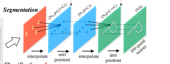
这里主要是进行上采样操作,但是由于点云是不规则的,所以无法直接使用普通的方式,具体实现代码如下:
class PointNetFeaturePropagation(nn.Module):
    def __init__(self, in_channel, mlp):
        """
        初始化函数,构建用于特征传播(上采样)的MLP层

        参数:
            in_channel: 输入特征的通道数(维度)
            mlp: 一个列表,表示每一层MLP的输出通道数,例如 [64, 128]
        """
        super(PointNetFeaturePropagation, self).__init__()

        # 用于保存卷积层和批归一化层
        self.mlp_convs = nn.ModuleList()
        self.mlp_bns = nn.ModuleList()

        last_channel = in_channel  # 当前输入通道数初始化为in_channel

        # 构建MLP层:每个层是一个Conv1d + BatchNorm1d + ReLU
        for out_channel in mlp:
            self.mlp_convs.append(nn.Conv1d(last_channel, out_channel, 1))
            self.mlp_bns.append(nn.BatchNorm1d(out_channel))
            last_channel = out_channel  # 更新下一层的输入通道数

    def forward(self, xyz1, xyz2, points1, points2):
        """
        前向传播函数:将稀疏点集points2插值到密集点集xyz1的位置上

        参数:
            xyz1: 原始点坐标数据,形状 [B, C, N] (如 1024 个点)
            xyz2: 下采样后的点坐标数据,形状 [B, C, S] (如 256 个点)
            points1: 原始点对应的特征数据,形状 [B, D, N] (可为 None)
            points2: 下采样点对应的特征数据,形状 [B, D, S]

        返回:
            new_points: 插值并融合后的特征,形状 [B, D', N]
        """
        # 将坐标和特征从 [B, C, N] 转换为 [B, N, C] 格式,便于后续计算
        xyz1 = xyz1.permute(0, 2, 1)     # [B, N, C]
        xyz2 = xyz2.permute(0, 2, 1)     # [B, S, C]
        points2 = points2.permute(0, 2, 1)  # [B, S, D]

        B, N, C = xyz1.shape             # 原始点数量 N
        _, S, _ = xyz2.shape             # 下采样点数量 S

        # 如果只有1个下采样点,直接复制其特征到所有原始点
        if S == 1:
            interpolated_points = points2.repeat(1, N, 1)  # [B, N, D]

        else:
            # 计算原始点与下采样点之间的距离矩阵(欧氏距离平方)
            dists = square_distance(xyz1, xyz2)  # [B, N, S]

            # 对每个原始点,找到最近的3个邻近点
            dists, idx = dists.sort(dim=-1)
            dists = dists[:, :, :3]   # 取最小的三个距离 [B, N, 3]
            idx = idx[:, :, :3]       # 取对应的索引 [B, N, 3]

            # 使用反距离加权(IDW)计算权重:
            # 1.将距离转换为“权重”,距离越近,权重越大
            dist_recip = 1.0 / (dists + 1e-8)  # 避免除以零
            # 2.对每个点的3个权重求和,得到归一化因子
            norm = torch.sum(dist_recip, dim=2, keepdim=True)  # 归一化因子
            # 3.归一化权重,使得每个点的权重之和为1
            weight = dist_recip / norm  # 加权平均系数 [B, N, 3]

            # 为每个原始点,找到它最近的 3 个邻近点,根据距离分配权重,然后对它们的特征做加权平均,从而插值得到该点的特征。
            # index_points: [B, S, D] -> [B, N, 3, D]
            # weight.view(B, N, 3, 1): 扩展维度后相乘
            interpolated_points = torch.sum(
                # 1. 从下采样点中取出每个原始点对应的最近邻点的特征。
                #    points2: [B, S, D] —— 下采样点的特征(S 个点,每个点有 D 维特征)
                #    idx: [B, N, 3] —— 每个原始点对应的 3 个最近邻点索引
                #    [B, N, 3, D] —— 每个原始点都有了它最近的 3 个邻近点的特征
                index_points(points2, idx)
                # 将之前计算好的权重扩展维度,以便和特征相乘。
                # weight: [B, N, 3] —— 每个点的三个邻近点的权重
                # [B, N, 3, 1] —— 扩展后便于广播乘法
                * weight.view(B, N, 3, 1),
                dim=2
            )  # [B, N, D]

        # 如果原始点有特征,则拼接起来(skip connection)
        if points1 is not None:
            points1 = points1.permute(0, 2, 1)  # [B, N, D]
            new_points = torch.cat([points1, interpolated_points], dim=-1)  # [B, N, D1+D2]
        else:
            new_points = interpolated_points  # [B, N, D]

        # 恢复张量格式为 [B, D, N],以适配后面的卷积操作
        new_points = new_points.permute(0, 2, 1)  # [B, D', N]

        # 经过MLP进一步提取和融合特征
        for i, conv in enumerate(self.mlp_convs):
            bn = self.mlp_bns[i]
            new_points = F.relu(bn(conv(new_points)))  # Conv1d + BN + ReLU

        return new_points  # 最终输出特征 [B, D', N]
这是类似图像中上采样的操作。
语义分割
语义分割的代码是先编码(使用编码器从1024-->256-->64-->16),然后进行解码,也就是我们刚刚所讲的类似上采样部分(从64-->256-->1024-->4096),主要功能是对输入点云中的每个点进行分类(如桌子、椅子、地板等),输出每个点的类别概率。
它的流程如下
1、使用 Set Abstraction(SA)层 进行多尺度特征提取和下采样;
2、使用 Feature Propagation(FP)层 进行特征插值和上采样;
3、最后通过两个卷积层输出每个点的分类结果;
4、输出为 [B, N, num_classes],即每个点都有一个类别预测。
class get_model(nn.Module):
    def __init__(self, num_classes):
        """
        初始化 PointNet++ 分割网络

        参数:
            num_classes: 分类类别数
        """
        super(get_model, self).__init__()

        # Set Abstraction 层(编码器部分)
        # 每层逐步下采样,并提取更高级别的局部特征
        self.sa1 = PointNetSetAbstraction(npoint=1024, radius=0.1, nsample=32, in_channel=9+3, mlp=[32, 32, 64], group_all=False)
        self.sa2 = PointNetSetAbstraction(npoint=256, radius=0.2, nsample=32, in_channel=64+3, mlp=[64, 64, 128], group_all=False)
        self.sa3 = PointNetSetAbstraction(npoint=64, radius=0.4, nsample=32, in_channel=128+3, mlp=[128, 128, 256], group_all=False)
        self.sa4 = PointNetSetAbstraction(npoint=16, radius=0.8, nsample=32, in_channel=256+3, mlp=[256, 256, 512], group_all=False)

        # Feature Propagation 层(解码器部分)
        # 从稀疏点恢复到原始点密度,逐层融合上下文信息
        self.fp4 = PointNetFeaturePropagation(in_channel=768, mlp=[256, 256])
        self.fp3 = PointNetFeaturePropagation(in_channel=384, mlp=[256, 256])
        self.fp2 = PointNetFeaturePropagation(in_channel=320, mlp=[256, 128])
        self.fp1 = PointNetFeaturePropagation(in_channel=128, mlp=[128, 128, 128])

        # 最终分类头
        self.conv1 = nn.Conv1d(128, 128, 1)
        self.bn1 = nn.BatchNorm1d(128)
        self.drop1 = nn.Dropout(0.5)
        self.conv2 = nn.Conv1d(128, num_classes, 1)

    def forward(self, xyz):
        """
        前向传播函数

        输入:
            xyz: 点云数据,形状 [B, C, N]

        返回:
            x: 每个点的分类结果,形状 [B, N, num_classes]
            l4_points: 最后一层抽象特征,用于其他任务
        """
        # l0 表示最原始的点云
        l0_points = xyz
        l0_xyz = xyz[:, :3, :]  # 只取 xyz 坐标,不带法向量或其他属性

        # 编码器:层层下采样并提取特征
        l1_xyz, l1_points = self.sa1(l0_xyz, l0_points)  # 1024 points
        l2_xyz, l2_points = self.sa2(l1_xyz, l1_points)  # 256 points
        l3_xyz, l3_points = self.sa3(l2_xyz, l2_points)  # 64 points
        l4_xyz, l4_points = self.sa4(l3_xyz, l3_points)  # 16 points

        # 解码器:层层插值并融合特征
        l3_points = self.fp4(l3_xyz, l4_xyz, l3_points, l4_points)  # 64 → 64
        l2_points = self.fp3(l2_xyz, l3_xyz, l2_points, l3_points)  # 256 → 256
        l1_points = self.fp2(l1_xyz, l2_xyz, l1_points, l2_points)  # 1024 → 1024
        l0_points = self.fp1(l0_xyz, l1_xyz, None, l1_points)       # 4096 → 4096

        # MLP 头部处理:进一步增强特征
        x = self.drop1(F.relu(self.bn1(self.conv1(l0_points)), inplace=True))  # [B, 128, N]
        x = self.conv2(x)  # [B, num_classes, N]

        # Softmax 分类
        x = F.log_softmax(x, dim=1)  # [B, num_classes, N]

        # 调整维度,返回 [B, N, num_classes]
        x = x.permute(0, 2, 1)

        return x, l4_points  # 返回每个点的分类结果和抽象特征
部件分割
部件分割与语义分割的主要区别如下:
1、部件分割使用了三层解码器,而语义分割是四层。
2、部件分割使用了全局特征,而语义分割则是主要依赖多层次局部特征。
3、部件分割要物体类别信息来区分部件语义,而语义分割不需要。
它的工作流程是使用SA层编码(512->128->1),而后再进行上采样(1->128->512),其他流程与语义分割类似
class get_model(nn.Module):
    def __init__(self, num_classes, normal_channel=False):
        super(get_model, self).__init__()
        if normal_channel:
            additional_channel = 3
        else:
            additional_channel = 0
        self.normal_channel = normal_channel
        self.sa1 = PointNetSetAbstraction(npoint=512, radius=0.2, nsample=32, in_channel=6+additional_channel, mlp=[64, 64, 128], group_all=False)
        self.sa2 = PointNetSetAbstraction(npoint=128, radius=0.4, nsample=64, in_channel=128 + 3, mlp=[128, 128, 256], group_all=False)
        self.sa3 = PointNetSetAbstraction(npoint=None, radius=None, nsample=None, in_channel=256 + 3, mlp=[256, 512, 1024], group_all=True)
        self.fp3 = PointNetFeaturePropagation(in_channel=1280, mlp=[256, 256])
        self.fp2 = PointNetFeaturePropagation(in_channel=384, mlp=[256, 128])
        self.fp1 = PointNetFeaturePropagation(in_channel=128+16+6+additional_channel, mlp=[128, 128, 128])
        self.conv1 = nn.Conv1d(128, 128, 1)
        self.bn1 = nn.BatchNorm1d(128)
        self.drop1 = nn.Dropout(0.5)
        self.conv2 = nn.Conv1d(128, num_classes, 1)

    def forward(self, xyz, cls_label):
        # Set Abstraction layers
        B,C,N = xyz.shape
        if self.normal_channel:
            l0_points = xyz
            l0_xyz = xyz[:,:3,:]
        else:
            l0_points = xyz
            l0_xyz = xyz
        l1_xyz, l1_points = self.sa1(l0_xyz, l0_points)
        l2_xyz, l2_points = self.sa2(l1_xyz, l1_points)
        l3_xyz, l3_points = self.sa3(l2_xyz, l2_points)
        # Feature Propagation layers
        l2_points = self.fp3(l2_xyz, l3_xyz, l2_points, l3_points)
        l1_points = self.fp2(l1_xyz, l2_xyz, l1_points, l2_points)
        #将物体类别标签转换为与点云相同维度的one-hot编码,用于条件特征融合。
        cls_label_one_hot = cls_label.view(B,16,1).repeat(1,1,N)
        l0_points = self.fp1(l0_xyz, l1_xyz, torch.cat([cls_label_one_hot,l0_xyz,l0_points],1), l1_points)
        # FC layers
        feat =  F.relu(self.bn1(self.conv1(l0_points)))
        x = self.drop1(feat)
        x = self.conv2(x)
        x = F.log_softmax(x, dim=1)
        x = x.permute(0, 2, 1)
        return x, l3_points
代码复现
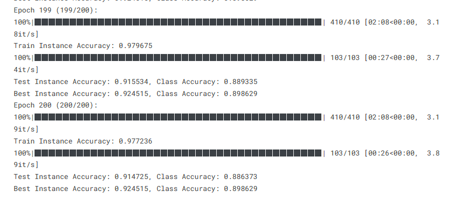
分类
在train_classfication中指定数据集,需要使用的数据集是modelnet40
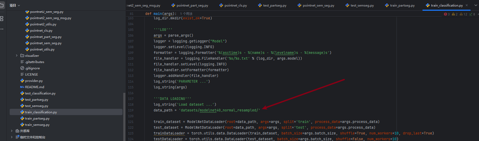
默认训练方式
python train_classification.py --model pointnet2_cls_ssg --log_dir pointnet2_cls_ssg
添加法向量的训练方式
python train_classification.py --model pointnet2_cls_ssg --use_normals --log_dir pointnet2_cls_ssg_normal
均匀采样方式
python train_classification.py --model pointnet2_cls_ssg --use_uniform_sample --log_dir pointnet2_cls_ssg_fps
分割
部件分割
这里使用的是ShapenNet数据集
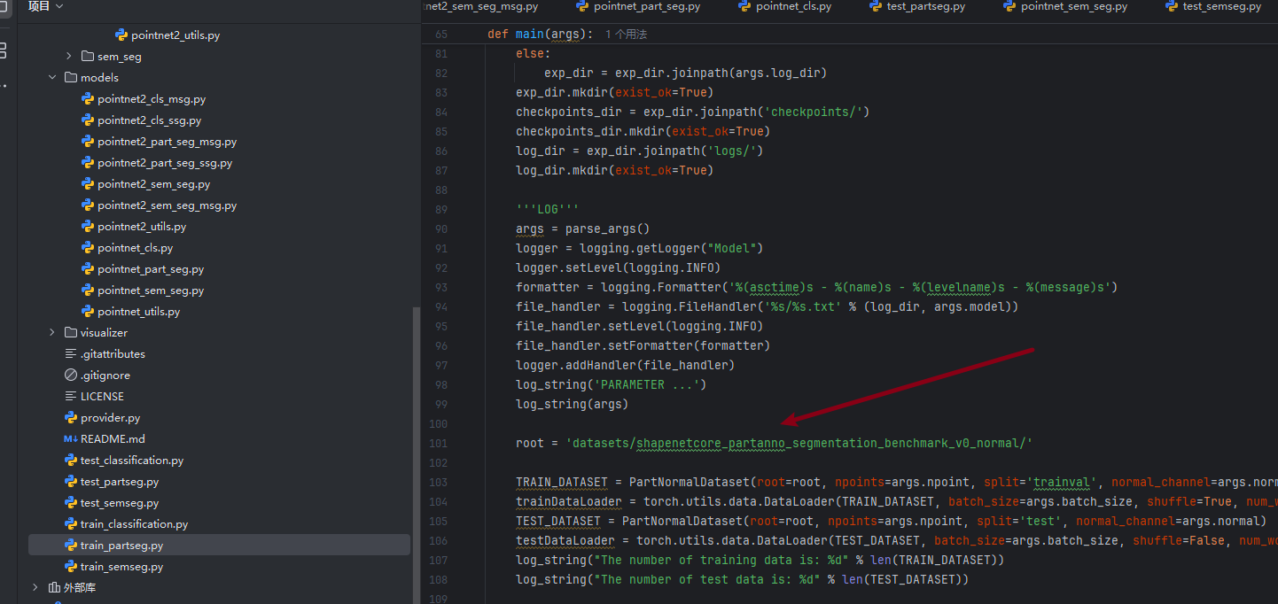
使用最新的numpy跟之前的代码有部分冲突,在train_partseg中的np.float后加上64即可
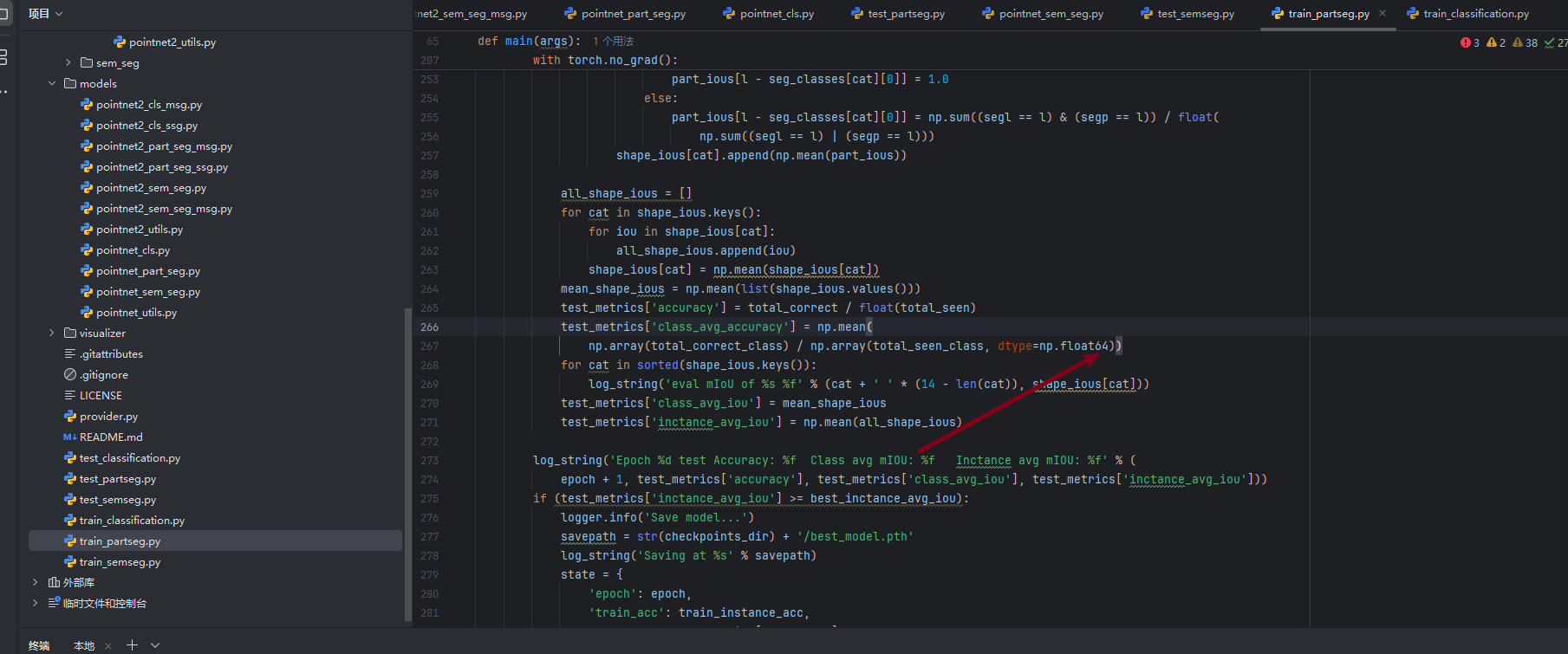
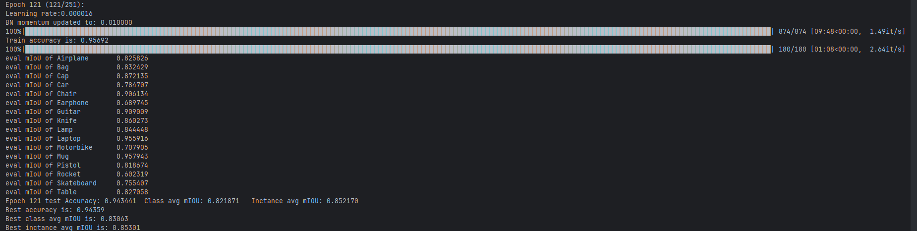
python train_partseg.py --model pointnet2_part_seg_msg --normal --log_dir pointnet2_part_seg_msg
训练效果如下
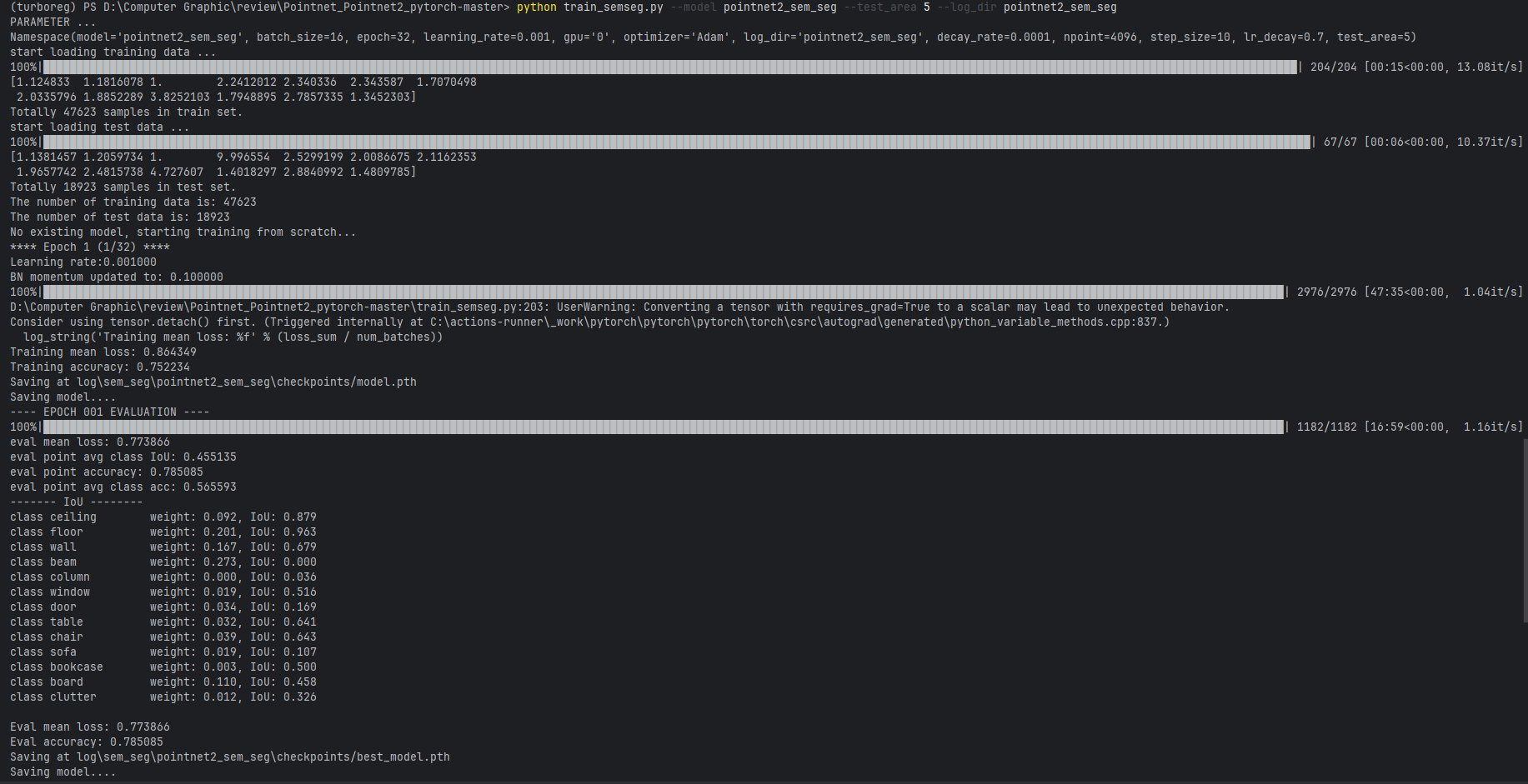
语义分割
这里使用的是S3DIS数据集,首先需要用collect_indoor3d_data进行处理,将此数据集改造为适合Pointnet++的数据集,将txt文本改为npy文件。
cd data_utils
python collect_indoor3d_data.py
然后将npy文件防止data/stanford_indoor3d下即可,数据库设置正确,即可运行代码进行语义分割测试
python train_semseg.py --model pointnet2_sem_seg --test_area 5 --log_dir pointnet2_sem_seg
python test_semseg.py --log_dir pointnet2_sem_seg --test_area 5 --visual
之后会生成obj文件,使用下面代码实现可视化
import open3d as o3d
import numpy as np


def visual_obj(path):
    with open(path, "r") as obj_file:
        points = []
        colors = []

        for line in obj_file.readlines():
            line = line.strip()
            line_list = line.split(" ")
            points.append(np.array(line_list[1:4]))
            colors.append(np.array(line_list[4:7]))

        pcd = o3d.geometry.PointCloud()
        pcd.points = o3d.utility.Vector3dVector(points)
        pcd.colors = o3d.utility.Vector3dVector(colors)
        o3d.visualization.draw_geometries([pcd])


def main():
    objt_file_path = r"D:\Computer Graphic\review\Pointnet_Pointnet2_pytorch-master\log\sem_seg\pointnet2_sem_seg\visual\Area_5_office_1_pred.obj"
    visual_obj(objt_file_path)


if __name__ == '__main__':
    main()
效果如下(这里是办公室的分割图)

Reference
https://blog.csdn.net/m0_51496369/article/details/145287243
https://blog.csdn.net/weixin_45144684/article/details/132012263
https://blog.csdn.net/m0_46677695/article/details/144246479
https://binaryoracle.github.io/3DVL/简析PointNet__.html

 浙公网安备 33010602011771号