实验二：逻辑回归算法实验

【实验目的】

理解逻辑回归算法原理，掌握逻辑回归算法框架；
理解逻辑回归的sigmoid函数；
理解逻辑回归的损失函数；
针对特定应用场景及数据，能应用逻辑回归算法解决实际分类问题。

【实验内容】

1.根据给定的数据集，编写python代码完成逻辑回归算法程序，实现如下功能：

建立一个逻辑回归模型来预测一个学生是否会被大学录取。假设您是大学部门的管理员，您想根据申请人的两次考试成绩来确定他们的入学机会。您有来自以前申请人的历史数据，可以用作逻辑回归的训练集。对于每个培训示例，都有申请人的两次考试成绩和录取决定。您的任务是建立一个分类模型，根据这两门考试的分数估计申请人被录取的概率。
算法步骤与要求：

(1)读取数据；(2)绘制数据观察数据分布情况；(3)编写sigmoid函数代码；(4)编写逻辑回归代价函数代码；(5)编写梯度函数代码；(6)编写寻找最优化参数代码（可使用scipy.opt.fmin_tnc()函数）；(7)编写模型评估（预测）代码，输出预测准确率；(8)寻找决策边界，画出决策边界直线图。

\2. 针对iris数据集，应用sklearn库的逻辑回归算法进行类别预测。

要求：

（1）使用seaborn库进行数据可视化；（2）将iri数据集分为训练集和测试集(两者比例为8:2)进行三分类训练和预测；（3）输出分类结果的混淆矩阵。

【实验报告要求】

对照实验内容，撰写实验过程、算法及测试结果；
代码规范化：命名规则、注释；
实验报告中需要显示并说明涉及的数学原理公式；
查阅文献，讨论逻辑回归算法的应用场景；

1. 读取数据

import pandas as pd
Data=pd.read_csv("ex2data1.txt",header=None,names=['Exam1', 'Exam2', 'Admitted'])
Data

	Exam1	Exam2	Admitted
0	34.623660	78.024693	0
1	30.286711	43.894998	0
2	35.847409	72.902198	0
3	60.182599	86.308552	1
4	79.032736	75.344376	1
5	45.083277	56.316372	0
6	61.106665	96.511426	1
7	75.024746	46.554014	1
8	76.098787	87.420570	1
9	84.432820	43.533393	1
10	95.861555	38.225278	0
11	75.013658	30.603263	0
12	82.307053	76.481963	1
13	69.364589	97.718692	1
14	39.538339	76.036811	0
15	53.971052	89.207350	1
16	69.070144	52.740470	1
17	67.946855	46.678574	0
18	70.661510	92.927138	1
19	76.978784	47.575964	1
20	67.372028	42.838438	0
21	89.676776	65.799366	1
22	50.534788	48.855812	0
23	34.212061	44.209529	0
24	77.924091	68.972360	1
25	62.271014	69.954458	1
26	80.190181	44.821629	1
27	93.114389	38.800670	0
28	61.830206	50.256108	0
29	38.785804	64.995681	0
...	...	...	...
70	32.722833	43.307173	0
71	64.039320	78.031688	1
72	72.346494	96.227593	1
73	60.457886	73.094998	1
74	58.840956	75.858448	1
75	99.827858	72.369252	1
76	47.264269	88.475865	1
77	50.458160	75.809860	1
78	60.455556	42.508409	0
79	82.226662	42.719879	0
80	88.913896	69.803789	1
81	94.834507	45.694307	1
82	67.319257	66.589353	1
83	57.238706	59.514282	1
84	80.366756	90.960148	1
85	68.468522	85.594307	1
86	42.075455	78.844786	0
87	75.477702	90.424539	1
88	78.635424	96.647427	1
89	52.348004	60.769505	0
90	94.094331	77.159105	1
91	90.448551	87.508792	1
92	55.482161	35.570703	0
93	74.492692	84.845137	1
94	89.845807	45.358284	1
95	83.489163	48.380286	1
96	42.261701	87.103851	1
97	99.315009	68.775409	1
98	55.340018	64.931938	1
99	74.775893	89.529813	1

100 rows × 3 columns

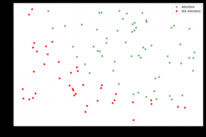
2. 数据分布状况

import matplotlib.pyplot as plt
#将录取和未录取进行分类
positive=Data[Data["Admitted"]==1]
negative=Data[Data["Admitted"]==0]
fig,ax=plt.subplots(figsize=(12,8))#创建画布，设置画布的大小
ax.scatter(positive['Exam1'],positive['Exam2'],s=30,c='g',marker='x',label='Admitted')#散点图，添加配置项
ax.scatter(negative['Exam1'],negative['Exam2'],s=30,c='r',marker='o',label='Not Admitted')
ax.legend() # 添加图例
ax.set_xlabel('Exam1 Score')
ax.set_ylabel('Exam2 Score')#添加x,y轴标签

Text(0,0.5,'Exam2 Score')

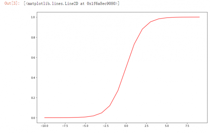
3. sigmoid函数

import numpy as np
def sigmoid(z):
    return 1/(1+np.exp(-z))
nums=np.arange(-10,10,step=1)
fig,ax=plt.subplots(figsize=(12,8))#设置画布的大小
ax.plot(nums,sigmoid(nums),"r")#在坐标轴上画线

4. logistics回归代价函数

def model(x,theta):
    return sigmoid(np.dot(x,theta.T))#dot矩阵的乘法运算 T转置

def cost(theta,x,y):
    theta = np.matrix(theta) #参数theta是一维数组，进行矩阵想乘时要把theta先转换为矩阵
    L1=np.multiply(-y,np.log(model(x,theta)))#multiply()数组和矩阵对应位置相乘
    L2=np.multiply(1-y,np.log(1-model(x,theta)))
    return np.sum(L1-L2)/(len(x))

Data.insert(0, 'Ones', 1)
cols=Data.shape[1]
x=np.array(Data.iloc[:,0:cols-1])#1-倒数第1列的数据
y=np.array(Data.iloc[:,cols-1:cols])#倒数第1列的数据
theta=np.zeros(x.shape[1])#1行三列的矩阵全部填充为0
print(cost(theta,x,y))

0.6931471805599453

5. 求梯度

def gradient(theta,x,y):
    theta = np.matrix(theta) #要先把theta转化为矩阵
    grad=np.dot(((model(x,theta)-y).T),x)/len(x)
    return np.array(grad).flatten()#因为下面寻找最优化参数的函数（opt.fmin_tnc())要求传入的gradient函返回值需要是一维数组，
                                   #因此需要利用flatten（）将grad进行转换以下 
gradient(theta,x,y)

array([ -0.1       , -12.00921659, -11.26284221])

6. 搜索最优化参数

import scipy.optimize as opt
result = opt.fmin_tnc(func=cost, x0=theta, fprime=gradient, args=(x, y))
result

(array([-25.16131864,   0.20623159,   0.20147149]), 36, 0)

7. 预测准确率

def predict(theta,x):
    theta=np.matrix(theta)
    temp=sigmoid(x*theta.T)
    return [1 if x >= 0.5 else 0 for x in temp]
theta=result[0]
predictValues=predict(theta,x)
hypothesis=[1 if a==b else 0 for (a,b)in zip(predictValues,y)]
accuracy=hypothesis.count(1)/len(hypothesis)
print ('accuracy = {0}%'.format(accuracy*100))

accuracy = 89.0%

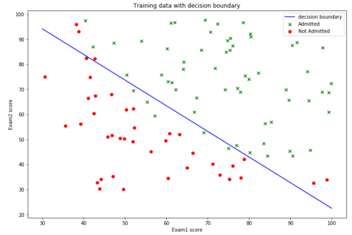
8. 得到决策边界并绘制

def find_x2(x1,theta):
    return [(-theta[0]-theta[1]*x_1)/theta[2] for x_1 in x1]
x1=np.linspace(30,100,1000)
x2=find_x2(x1,theta)
Data1=Data[Data['Admitted']==1]
Data2=Data[Data['Admitted']==0]
fig,ax=plt.subplots(figsize=(12,8))
ax.scatter(Data1['Exam1'],Data1['Exam2'],c='g',marker='x',label='Admitted')
ax.scatter(Data2['Exam2'],Data2['Exam1'],c='r',marker='o',label="Not Admitted")
ax.plot(x1,x2,'b',label="decision boundary")
ax.legend(loc=1)
ax.set_xlabel('Exam1 score')
ax.set_ylabel('Exam2 score')
ax.set_title("Training data with decision boundary")
plt.show()

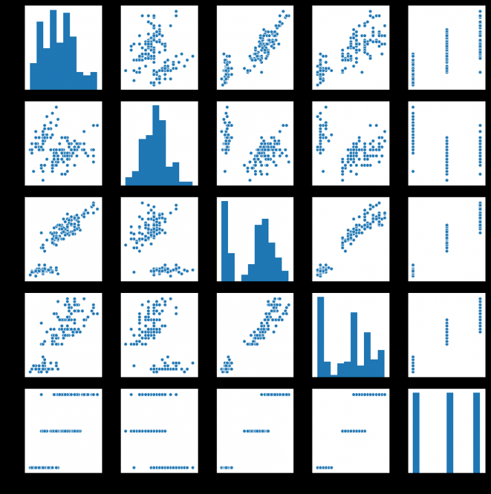
9. 对iris数据集数据分析

import seaborn as sns
from sklearn.datasets import load_iris# 我们利用 sklearn 中自带的 iris 数据作为数据载入，并利用Pandas转化为DataFrame格式
data=load_iris() #得到数据特征
iris_target=data.target #得到数据对应的标签
iris_features=pd.DataFrame(data=data.data, columns=data.feature_names) #利用Pandas转化为DataFrame格式
iris_features.describe()
iris_all=iris_features.copy()
iris_all['target']=iris_target
#利用value_counts函数查看每个类别数量
pd.Series(iris_target).value_counts()
sns.pairplot(data=iris_all) # pairplot用来进行数据分析，画两两特征图。
plt.show()

10. 对iris数据集调用sk-learn的logistics回归进行类别预测

from sklearn.model_selection import train_test_split
X_train,X_test,y_train,y_test = train_test_split(iris_features,iris_target,test_size=0.3)
from sklearn.linear_model import LogisticRegression
clf=LogisticRegression(random_state=0,solver='lbfgs')
# 在训练集上训练逻辑回归模型
clf.fit(X_train,y_train)
print('the weight of Logistic Regression:\n',clf.coef_)
print('the intercept(w0) of Logistic Regression:\n',clf.intercept_)
train_predict=clf.predict(X_train)
test_predict=clf.predict(X_test)

the weight of Logistic Regression:
 [[-0.39310536  0.77102865 -2.124489   -0.91813939]
 [-0.28361972 -1.80748255  0.69900858 -1.23623074]
 [-0.32296799 -0.38952886  2.55652139  2.16024956]]
the intercept(w0) of Logistic Regression:
 [  6.20645518   5.06911911 -12.89262715]

11. 将iris数据集分0.7训练集0.3测试集进行三分类训练和预测

from sklearn.model_selection import train_test_split
X_train,X_test,y_train,y_test = train_test_split(iris_features,iris_target,test_size=0.3)
from sklearn.linear_model import LogisticRegression
clf=LogisticRegression(random_state=0,solver='lbfgs')
# 在训练集上训练逻辑回归模型
clf.fit(X_train,y_train)
print('the weight of Logistic Regression:\n',clf.coef_)
print('the intercept(w0) of Logistic Regression:\n',clf.intercept_)
train_predict=clf.predict(X_train)
test_predict=clf.predict(X_test)

the weight of Logistic Regression:
 [[-0.39310536  0.77102865 -2.124489   -0.91813939]
 [-0.28361972 -1.80748255  0.69900858 -1.23623074]
 [-0.32296799 -0.38952886  2.55652139  2.16024956]]
the intercept(w0) of Logistic Regression:
 [  6.20645518   5.06911911 -12.89262715]

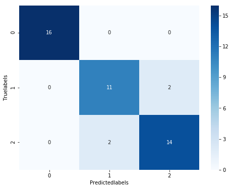
12. 输出iris数据集分类结果的confusion matrix

from sklearn import metrics
#利用accuracy（准确度）【预测正确的样本数目占总预测样本数目的比例】评估模型效果
print('The accuracy of the Logistic Regression is:',metrics.accuracy_score(y_train,train_predict))
print('The accuracy of the Logistic Regression is:',metrics.accuracy_score(y_test,test_predict))
#查看混淆矩阵(预测值和真实值的各类情况统计矩阵)
confusion_matrix_result=metrics.confusion_matrix(y_test,test_predict)
print('The confusion matrix result:\n',confusion_matrix_result)
# 利用热力图对于结果进行可视化,画混淆矩阵
plt.figure(figsize=(8,6))
sns.heatmap(confusion_matrix_result,annot=True,cmap='Reds')
plt.xlabel('Predictedlabels')
plt.ylabel('Truelabels')
plt.show()

The accuracy of the Logistic Regression is: 0.9583333333333334
The accuracy of the Logistic Regression is: 0.8
The confusion matrix result:
 [[10  0  0]
 [ 0  7  3]
 [ 0  3  7]]

13. 算法涉及的数学原理

（1）sigmoid

\[y=f(x)=\frac{1}{1+e^{-x} } \]

（2）梯度下降

\[J(\theta)=\frac{1}{2}\left[h_{t}(x)-y\right]^{2} \]

\[\frac{\partial J}{\partial \theta_{j}}=-\frac{1}{m} \sum_{i=1}^{n}\left(y_{i}-h_{\theta}\left(x_{i}\right)\right) x_{i j} \]

\[\begin{array}{l} l(\theta)=\log L(\theta)=\sum_{i=1}\left(y_{i} \log h_{\theta}\left(x_{i}\right)+\left(1-y_{i}\right) \log \left(1-h_{\theta}\left(x_{i}\right)\right)\right) \\ \frac{\delta}{\delta_{\theta}} J(\theta)=-\frac{1}{m} \sum_{i=1}^{m}\left(y_{i} \frac{1}{h_{\theta}\left(x_{i}\right)} \frac{\delta}{\delta_{\theta}} h_{\theta}\left(x_{i}\right)-\left(1-\mathrm{y}_{\mathrm{i}}\right) \frac{1}{1-h_{\theta}\left(x_{i}\right)} \frac{\delta}{\delta_{\theta}} h_{\theta}\left(x_{i}\right)\right) \\ =-\frac{1}{m} \sum_{i=1}^{m}\left(y_{i} \frac{1}{g\left(\theta^{\mathrm{T}} x_{i}\right)}-\left(1-\mathrm{y}_{\mathrm{i}}\right) \frac{1}{1-g\left(\theta^{\mathrm{T}} x_{i}\right)}\right) \frac{\delta}{\delta_{\theta}} g\left(\theta^{\mathrm{T}} x_{i}\right) \\ =-\frac{1}{m} \sum_{i=1}^{m}\left(y_{i} \frac{1}{g\left(\theta^{\mathrm{T}} x_{i}\right)}-\left(1-\mathrm{y}_{\mathrm{i}}\right) \frac{1}{1-g\left(\theta^{\mathrm{T}} x_{i}\right)}\right) g\left(\theta^{\mathrm{T}} x_{i}\right)\left(1-g\left(\theta^{\mathrm{T}} x_{i}\right)\right) \frac{\delta}{\delta_{\theta}} \theta^{\mathrm{T}} x_{i} \\ =-\frac{1}{m} \sum_{i=1}^{m}\left(y_{i}\left(1-g\left(\theta^{\mathrm{T}} x_{i}\right)\right)-\left(1-\mathrm{y}_{\mathrm{i}}\right) g\left(\theta^{\mathrm{T}} x_{i}\right)\right) x_{i}^{j} \\ =-\frac{1}{m} \sum_{i=1}^{m}\left(y_{i}-g\left(\theta^{\mathrm{T}} x_{i}\right)\right) x_{i}^{j} \\ =\frac{1}{m} \sum_{i=1}^{m}\left(h_{\theta}\left(x_{i}\right)-y_{i}\right) x_{i}^{j} \end{array} \]

\[\theta_{n+1}=\theta_{n}-\alpha J^{\prime}(\theta) \]

（3）损失函数

\[J(\theta)=\frac{1}{m} \sum_{i=1}^{m} \operatorname{Cos} t\left(h_{\theta}\left(x^{(i)}\right), y^{(i)}\right) \]

\[J(\theta)=\frac{1}{m} \sum_{i=1}^{m} \operatorname{Cos} t\left(h_{\theta}\left(x^{(i)}\right), y^{(i)}\right)\operatorname{Cost}\left(h_{\theta}(x), y\right)=\left\{\begin{aligned} -\log \left(h_{\theta}(x)\right) & \text { if } y=1 \\ -\log \left(1-h_{\theta}(x)\right) & \text { if } y=0 \end{aligned}\right. \]

14. 逻辑回归算法的应用场景

1. 用于分类场景， 尤其是因变量是二分类（0/1，True/False，Yes/No）时我们应该使用逻辑回归。
2. 不要求自变量和因变量是线性关系

15. 存在的问题

1. 防止过拟合和低拟合，应该让模型构建的变量是显著的。一个好的方法是使用逐步回归方法去进行逻辑回归。
2. 逻辑回归需要大样本量，因为最大似然估计在低样本量的情况下不如最小二乘法有效。
3. 独立的变量要求没有共线性。