机器学习sklearn（68）：算法实例（二十五）分类（十二）SVM（三）sklearn.svm.SVC（二）

2 非线性SVM与核函数

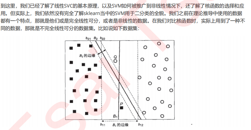
2.1 SVC在非线性数据上的推广

 

 

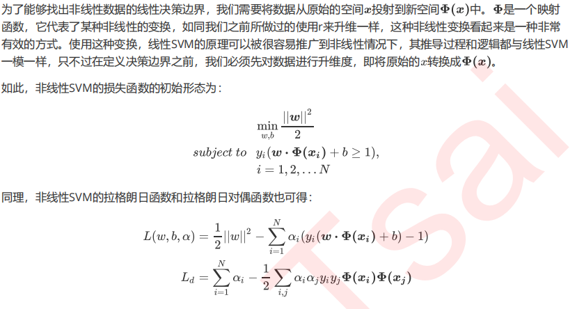
2.2 重要参数kernel

 

 

 

 

 

 

clf = SVC(kernel = "rbf").fit(X,y)
plt.scatter(X[:,0],X[:,1],c=y,s=50,cmap="rainbow")
plot_svc_decision_function(clf)

可以看到，决策边界被完美地找了出来。

2.3 探索核函数在不同数据集上的表现

 

 

1. 导入所需要的库和模块

import numpy as np
import matplotlib.pyplot as plt
from matplotlib.colors import ListedColormap
from sklearn import svm
from sklearn.datasets import make_circles, make_moons, make_blobs,make_classification

2. 创建数据集，定义核函数的选择 

n_samples = 100
datasets = [
    make_moons(n_samples=n_samples, noise=0.2, random_state=0),
    make_circles(n_samples=n_samples, noise=0.2, factor=0.5, random_state=1),
    make_blobs(n_samples=n_samples, centers=2, random_state=5),
    make_classification(n_samples=n_samples,n_features = 
2,n_informative=2,n_redundant=0, random_state=5)
 ]
Kernel = ["linear","poly","rbf","sigmoid"] 

#四个数据集分别是什么样子呢？
for X,Y in datasets:
    plt.figure(figsize=(5,4))
    plt.scatter(X[:,0],X[:,1],c=Y,s=50,cmap="rainbow")

3. 构建子图 

nrows=len(datasets)
ncols=len(Kernel) + 1
fig, axes = plt.subplots(nrows, ncols,figsize=(20,16))

4. 开始进行子图循环

#第一层循环：在不同的数据集中循环
for ds_cnt, (X,Y) in enumerate(datasets):
    
    #在图像中的第一列，放置原数据的分布
    ax = axes[ds_cnt, 0]
    if ds_cnt == 0:
        ax.set_title("Input data")
    ax.scatter(X[:, 0], X[:, 1], c=Y, zorder=10, cmap=plt.cm.Paired,edgecolors='k')
    ax.set_xticks(())
    ax.set_yticks(())
    
    #第二层循环：在不同的核函数中循环
    #从图像的第二列开始，一个个填充分类结果
    for est_idx, kernel in enumerate(Kernel):
        
        #定义子图位置
        ax = axes[ds_cnt, est_idx + 1]
        
        #建模
        clf = svm.SVC(kernel=kernel, gamma=2).fit(X, Y)
        score = clf.score(X, Y)
        
        #绘制图像本身分布的散点图
        ax.scatter(X[:, 0], X[:, 1], c=Y
                   ,zorder=10
                   ,cmap=plt.cm.Paired,edgecolors='k')
        #绘制支持向量
        ax.scatter(clf.support_vectors_[:, 0], clf.support_vectors_[:, 1], s=50,
                    facecolors='none', zorder=10, edgecolors='k')
        
        #绘制决策边界
        x_min, x_max = X[:, 0].min() - .5, X[:, 0].max() + .5
        y_min, y_max = X[:, 1].min() - .5, X[:, 1].max() + .5
        
        #np.mgrid，合并了我们之前使用的np.linspace和np.meshgrid的用法
        #一次性使用最大值和最小值来生成网格
        #表示为[起始值：结束值：步长]
        #如果步长是复数，则其整数部分就是起始值和结束值之间创建的点的数量，并且结束值被包含在内
        XX, YY = np.mgrid[x_min:x_max:200j, y_min:y_max:200j]
        #np.c_，类似于np.vstack的功能
        Z = clf.decision_function(np.c_[XX.ravel(), YY.ravel()]).reshape(XX.shape)
        #填充等高线不同区域的颜色
        ax.pcolormesh(XX, YY, Z > 0, cmap=plt.cm.Paired)
        #绘制等高线
        ax.contour(XX, YY, Z, colors=['k', 'k', 'k'], linestyles=['--', '-', '--'],
                    levels=[-1, 0, 1])
        
        #设定坐标轴为不显示
        ax.set_xticks(())
        ax.set_yticks(())
        
        #将标题放在第一行的顶上
        if ds_cnt == 0:
            ax.set_title(kernel)
            
        #为每张图添加分类的分数   
        ax.text(0.95, 0.06, ('%.2f' % score).lstrip('0')
               , size=15
               , bbox=dict(boxstyle='round', alpha=0.8, facecolor='white')
               #为分数添加一个白色的格子作为底色
               , transform=ax.transAxes #确定文字所对应的坐标轴，就是ax子图的坐标轴本身
               , horizontalalignment='right' #位于坐标轴的什么方向
               )
plt.tight_layout()
plt.show()

 

 

2.4 探索核函数的优势和缺陷 

看起来，除了Sigmoid核函数，其他核函数效果都还不错。但其实rbf和poly都有自己的弊端，我们使用乳腺癌数据集作为例子来展示一下：

from sklearn.datasets import load_breast_cancer
from sklearn.svm import SVC
from sklearn.model_selection import train_test_split
import matplotlib.pyplot as plt
import numpy as np
from time import time
import datetime
data = load_breast_cancer()
X = data.data
y = data.target
X.shape
np.unique(y)
plt.scatter(X[:,0],X[:,1],c=y)
plt.show()
Xtrain, Xtest, Ytrain, Ytest = train_test_split(X,y,test_size=0.3,random_state=420)
Kernel = ["linear","poly","rbf","sigmoid"]
for kernel in Kernel:
    time0 = time()
    clf= SVC(kernel = kernel
             , gamma="auto"
            # , degree = 1
             , cache_size=5000
           ).fit(Xtrain,Ytrain)
    print("The accuracy under kernel %s is %f" % (kernel,clf.score(Xtest,Ytest)))
    print(datetime.datetime.fromtimestamp(time()-time0).strftime("%M:%S:%f"))

Kernel = ["linear","rbf","sigmoid"]

for kernel in Kernel:
    time0 = time()
    clf= SVC(kernel = kernel
             , gamma="auto"
            # , degree = 1
             , cache_size=5000
           ).fit(Xtrain,Ytrain)
    print("The accuracy under kernel %s is %f" % (kernel,clf.score(Xtest,Ytest)))
    print(datetime.datetime.fromtimestamp(time()-time0).strftime("%M:%S:%f"))

Kernel = ["linear","poly","rbf","sigmoid"]

for kernel in Kernel:
    time0 = time()
    clf= SVC(kernel = kernel
             , gamma="auto"
             , degree = 1
             , cache_size=5000
           ).fit(Xtrain,Ytrain)
    print("The accuracy under kernel %s is %f" % (kernel,clf.score(Xtest,Ytest)))
    print(datetime.datetime.fromtimestamp(time()-time0).strftime("%M:%S:%f"))

import pandas as pd
data = pd.DataFrame(X)
data.describe([0.01,0.05,0.1,0.25,0.5,0.75,0.9,0.99]).T

望去，果然数据存在严重的量纲不一的问题。我们来使用数据预处理中的标准化的类，对数据进行标准化： 

from sklearn.preprocessing import StandardScaler
X = StandardScaler().fit_transform(X)
data = pd.DataFrame(X)
data.describe([0.01,0.05,0.1,0.25,0.5,0.75,0.9,0.99]).T

标准化完毕后，再次让SVC在核函数中遍历，此时我们把degree的数值设定为1，观察各个核函数在去量纲后的数据上的表现： 

Xtrain, Xtest, Ytrain, Ytest = train_test_split(X,y,test_size=0.3,random_state=420)
Kernel = ["linear","poly","rbf","sigmoid"]
for kernel in Kernel:
    time0 = time()
    clf= SVC(kernel = kernel
             , gamma="auto"
             , degree = 1
             , cache_size=5000
           ).fit(Xtrain,Ytrain)
    print("The accuracy under kernel %s is %f" % (kernel,clf.score(Xtest,Ytest)))
    print(datetime.datetime.fromtimestamp(time()-time0).strftime("%M:%S:%f"))

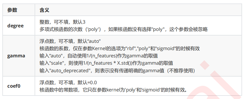
2.5 选取与核函数相关的参数：degree & gamma & coef0

 

 

score = []
gamma_range = np.logspace(-10, 1, 50) #返回在对数刻度上均匀间隔的数字
for i in gamma_range:
    clf = SVC(kernel="rbf",gamma = i,cache_size=5000).fit(Xtrain,Ytrain)
    score.append(clf.score(Xtest,Ytest))
    
print(max(score), gamma_range[score.index(max(score))])
plt.plot(gamma_range,score)
plt.show()

from sklearn.model_selection import StratifiedShuffleSplit
from sklearn.model_selection import GridSearchCV
time0 = time()
gamma_range = np.logspace(-10,1,20)
coef0_range = np.linspace(0,5,10)
param_grid = dict(gamma = gamma_range
                 ,coef0 = coef0_range)
cv = StratifiedShuffleSplit(n_splits=5, test_size=0.3, random_state=420)
grid = GridSearchCV(SVC(kernel = "poly",degree=1,cache_size=5000), 
param_grid=param_grid, cv=cv)
grid.fit(X, y)
print("The best parameters are %s with a score of %0.5f" % (grid.best_params_, 
grid.best_score_))
print(datetime.datetime.fromtimestamp(time()-time0).strftime("%M:%S:%f"))

3 硬间隔与软间隔：重要参数C 

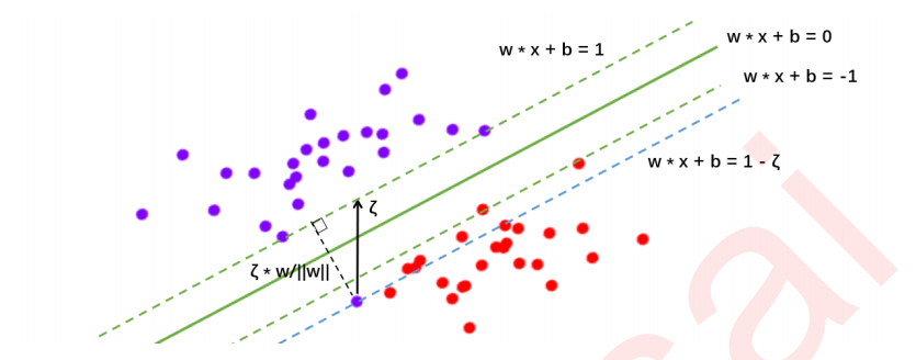
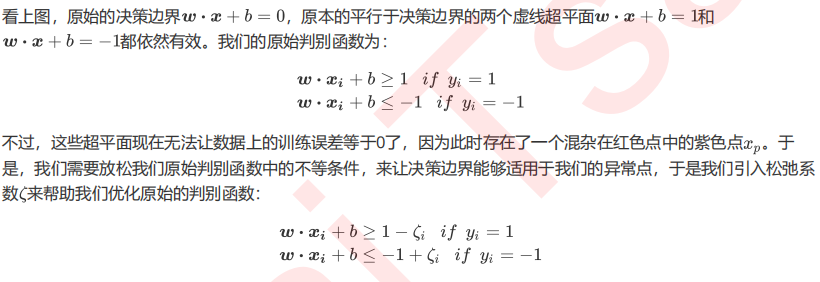
3.1 SVM在软间隔数据上的推广 

 

 

 

 

 

 

 

 

 

 

 

 

 

 

 

 

 

 

 

 

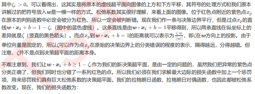
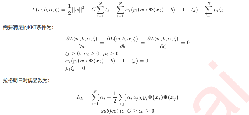
3.2 重要参数C 

 

 

 

 

#调线性核函数
score = []
C_range = np.linspace(0.01,30,50)
for i in C_range:
    clf = SVC(kernel="linear",C=i,cache_size=5000).fit(Xtrain,Ytrain)
    score.append(clf.score(Xtest,Ytest))
print(max(score), C_range[score.index(max(score))])
plt.plot(C_range,score)
plt.show()
#换rbf
score = []
C_range = np.linspace(0.01,30,50)
for i in C_range:
    clf = SVC(kernel="rbf",C=i,gamma = 
0.012742749857031322,cache_size=5000).fit(Xtrain,Ytrain)
    score.append(clf.score(Xtest,Ytest))
    
print(max(score), C_range[score.index(max(score))])
plt.plot(C_range,score)
plt.show()
#进一步细化
score = []
C_range = np.linspace(5,7,50)
for i in C_range:
    clf = SVC(kernel="rbf",C=i,gamma = 
0.012742749857031322,cache_size=5000).fit(Xtrain,Ytrain)
    score.append(clf.score(Xtest,Ytest))
    
print(max(score), C_range[score.index(max(score))])
plt.plot(C_range,score)
plt.show()

4 总结