


标签传播算法(llgc 或 lgc)
动手实践标签传播算法
复现论文:Learning with Local and Global Consistency[1]
lgc 算法可以参考:DecodePaper/notebook/lgc
初始化算法
载入一些必备的库:
from IPython.display import set_matplotlib_formats
%matplotlib inline
#set_matplotlib_formats('svg', 'pdf')

import numpy as np
import matplotlib.pyplot as plt
from scipy.spatial.distance import cdist
from sklearn.datasets import make_moons

save_dir = '../data/images'
创建一个简单的数据集
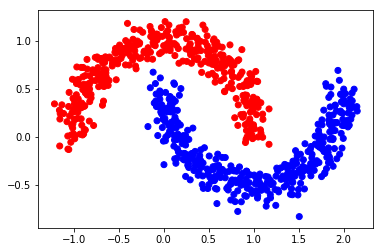
利用 make_moons 生成一个半月形数据集。
n = 800   # 样本数
n_labeled = 10 # 有标签样本数
X, Y = make_moons(n, shuffle=True, noise=0.1, random_state=1000)

X.shape, Y.shape
((800, 2), (800,))
def one_hot(Y, n_classes):
    '''
    对标签做 one_hot 编码

    参数
    =====
    Y: 从 0 开始的标签
    n_classes: 类别数
    '''
    out = Y[:, None] == np.arange(n_classes)
    return out.astype(float)
color = ['red' if l == 0 else 'blue' for l in Y]
plt.scatter(X[:, 0], X[:, 1], color=color)
plt.savefig(f"{save_dir}/bi_classification.pdf", format='pdf')
plt.show()

Y_input = np.concatenate((one_hot(Y[:n_labeled], 2), np.zeros((n-n_labeled, 2))))
算法过程:
Step 1: 创建相似度矩阵 W
def rbf(x, sigma):
    return np.exp((-x)/(2* sigma**2))
sigma = 0.2
dm = cdist(X, X, 'euclidean')
W = rbf(dm, sigma)
np.fill_diagonal(W, 0)   # 对角线全为 0
Step 2: 计算 S
\[S = D^{-\frac{1}{2}} W D^{-\frac{1}{2}}
\]
向量化编程:
def calculate_S(W):
    d = np.sum(W, axis=1)
    D_ = np.sqrt(d*d[:, np.newaxis]) # D_ 是 np.sqrt(np.dot(diag(D),diag(D)^T))
    return np.divide(W, D_, where=D_ != 0)


S = calculate_S(W)
迭代一次的结果
alpha = 0.99
F = np.dot(S, Y_input)*alpha + (1-alpha)*Y_input

Y_result = np.zeros_like(F)
Y_result[np.arange(len(F)), F.argmax(1)] = 1

Y_v = [1 if x == 0 else 0 for x in Y_result[0:,0]]

color = ['red' if l == 0 else 'blue' for l in Y_v]
plt.scatter(X[0:,0], X[0:,1], color=color)
#plt.savefig("iter_1.pdf", format='pdf')
plt.show()
Step 3: 迭代 F "n_iter" 次直到收敛
n_iter = 150
F = Y_input
for t in range(n_iter):
    F = np.dot(S, F)*alpha + (1-alpha)*Y_input
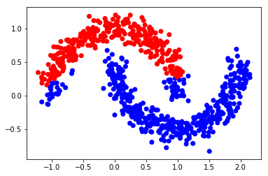
Step 4: 画出最终结果
Y_result = np.zeros_like(F)
Y_result[np.arange(len(F)), F.argmax(1)] = 1

Y_v = [1 if x == 0 else 0 for x in Y_result[0:,0]]

color = ['red' if l == 0 else 'blue' for l in Y_v]
plt.scatter(X[0:,0], X[0:,1], color=color)
#plt.savefig("iter_n.pdf", format='pdf')
plt.show()

from sklearn import metrics

print(metrics.classification_report(Y, F.argmax(1)))

acc = metrics.accuracy_score(Y, F.argmax(1))
print('准确度为',acc)
              precision    recall  f1-score   support

           0       1.00      0.86      0.92       400
           1       0.88      1.00      0.93       400

   micro avg       0.93      0.93      0.93       800
   macro avg       0.94      0.93      0.93       800
weighted avg       0.94      0.93      0.93       800

准确度为 0.92875
sklearn 实现 lgc
参考:https://scikit-learn.org/stable/modules/label_propagation.html
在 sklearn 里提供了两个 lgc 模型:LabelPropagation 和 LabelSpreading,其中后者是前者的正则化形式。\(W\) 的计算方式提供了 rbf 与 knn。
rbf核由参数gamma控制(\(\gamma=\frac{1}{2{\sigma}^2}\))knn核 由参数n_neighbors(近邻数)控制
def pred_lgc(X, Y, F, numLabels):
    from sklearn import preprocessing
    from sklearn.semi_supervised import LabelSpreading
    cls = LabelSpreading(max_iter=150, kernel='rbf', gamma=0.003, alpha=.99)
    # X.astype(float) 为了防止报错 "Numerical issues were encountered "
    cls.fit(preprocessing.scale(X.astype(float)), F)
    ind_unlabeled = np.arange(numLabels, len(X))
    y_pred = cls.transduction_[ind_unlabeled]
    y_true = Y[numLabels:].astype(y_pred.dtype)
    return y_true, y_pred
Y_input = np.concatenate((Y[:n_labeled], -np.ones(n-n_labeled)))
y_true, y_pred = pred_lgc(X, Y, Y_input, n_labeled)
print(metrics.classification_report(Y, F.argmax(1)))
              precision    recall  f1-score   support

           0       1.00      0.86      0.92       400
           1       0.88      1.00      0.93       400

   micro avg       0.93      0.93      0.93       800
   macro avg       0.94      0.93      0.93       800
weighted avg       0.94      0.93      0.93       800
networkx 实现 lgc
参考:networkx.algorithms.node_classification.lgc.local_and_global_consistency 具体的细节,我还没有研究!先放一个简单的例子:
G = nx.path_graph(4)
G.node[0]['label'] = 'A'
G.node[3]['label'] = 'B'
G.nodes(data=True)

G.edges()

predicted = node_classification.local_and_global_consistency(G)
predicted
['A', 'A', 'B', 'B']
更多精彩内容见:DecodePaper 觉得有用,记得给个 star !(@DecodePaper)
Zhou D, Bousquet O, Lal T N, et al. Learning with Local and Global Consistency[C]. neural information processing systems, 2003: 321-328. ↩︎
探寻有趣之事!

 浙公网安备 33010602011771号