day-11 python自带库实现2层简单神经网络算法

　　深度神经网络算法，是基于神经网络算法的一种拓展，其层数更深，达到多层，本文以简单神经网络为例，利用梯度下降算法进行反向更新来训练神经网络权重和偏向参数，文章最后，基于Python 库实现了一个简单神经网络算法程序，并对异或运算和0-9字符集进行预测。

一、问题引入

　　利用如下图像结构，通过训练集对其参数进行训练，当有新的测试数据时，通过更新函数，获得正确的预测值，更新函数方程为：

　　　　O_ij = activation(sum(x_i*w_ij)+b_ij)

　　图中为简单的两层神经网络结构，4,5对应的为隐藏层，6为输出层， activation代表激活函数，常用的有logistic和tanh函数，b称为偏向。

二、神经网络正向更新和反向更新规则介绍

　　对于正向更新：

　　　　O_ij = activation(sum(x_i*w_ij)+b_ij)

　　对于反向更新：

　　　　对于输出层：Err_j = activation_derivate(O_j)*(T_j-O_j)

　　　　对于隐藏层：Err_j = activation_derivate(O_j)*sum(Err_k*W_jk)

　　　　delta(W_ij) = l*Err_j*O_ij

　　　　delta(b_j) = l*Err_j

　　　　w_ij = w_ij + delta(w_ij)

　　　　b_j = b_j + delta(b_j)

　　其中:

　　　　j代表第j层

　　　　k代表输出层

　　　　T代表实际标记值

　　　　O代表输出值

　　　　activation代表激活函数，常用的有logistic和tanh函数

　　　　activation_derivate代表激活函数的倒数

三、一个简单神经网络的数学运算实例

　　我们以一个3×2×1神经网络为例，说明如何利用正向更新和反向更新来训练神经网络，完成一次更新：

x1	x2	x3	w14	w15	w24	w25	w34	w35	w46	w56	b4	b5	b6
1	0	1	0.2	-0.3	0.4	0.1	-0.5	0.2	-0.3	-0.2	-0.4	-0.2	0.1

　　同时，我们设定学习率l=0.9，实际输出值为1

 

import numpy as np
x1 = 1
x2 = 0
x3 = 1
w14 = 0.2
w15 = -0.3
w24 = 0.4
w25 = 0.1
w34 = -0.5
w35 = 0.2
w46 = -0.3
w56 = -0.2
b4 = -0.4
b5 = 0.2
b6 = 0.1
l = 0.9
t = 1
 
# 定义activation函数和倒数
def logistic(x):
    return 1/(1+np.exp(-x))
 
def logistic_derivate(x):
    return x*(1-x)
 
# 正向更新
z4 = x1*w14 + x2*w24 + x3*w34 + b4
z5 = x1*w15 + x2*w25 + x3*w35 + b5
O4 = logistic(z4)
O5 = logistic(z5)
z6 = O4*w46 + O5 * w56 + b6
O6 = logistic(z6)
print(O4,O5,O6)
结果：0.331812227832 0.524979187479 0.473888898824

# 求取各个神经元节点误差值
E6 = logistic_derivate(O6)*(t-O6)
E5 = logistic_derivate(O5)*E6*w56
E4 = logistic_derivate(O4)*E6*w46 
print(E6,E5,E4)
结果：0.131169078214 -0.00654208506417 -0.00872456196543

# 反向更新权重和偏向
w46 = w46 + l*E6*O4
w56 = w56 + l*E6*O5
w14 = w14 + l*E4*x1
w24 = w14 + l*E4*x2
w34 = w34 + l*E4*x3
w15 = w15 + l*E5*x1
w25 = w25 + l*E5*x2
w35 = w35 + l*E5*x3
print(w46,w56,w14,w15,w24,w25,w34,w35)
结果：-0.260828846342 -0.138025067507 0.192147894231 -0.305887876558 0.192147894231 0.1 -0.507852105769 0.194112123442

b4 = b4 + l*E4
b5 = b5 + l*E5
b6 = b6 + l*E6
print(b4,b5,b6)
结果：-0.407852105769 0.194112123442 0.21805217039

 

 

 

四、简单神经网络算python实现程序

　　介绍程序前，首先引入一个矩阵点乘基本运算

import numpy as np


# 一维矩阵

a = np.arange(0,9)

print(a)

b = a[::-1]

print(b)

print(np.dot(a,b))


# 二维矩阵

a = np.arange(1,5).reshape(2,2)

print(a)

b = np.arange(5,9).reshape(2,2)

print(b)

c = np.dot(a,b)

print(c)


结果：

[0 1 2 3 4 5 6 7 8]

[8 7 6 5 4 3 2 1 0]

84

[[1 2]

[3 4]]

[[5 6]

[7 8]]

[[19 22]

[43 50]]

　　在实际编程过程中，引入7,8节点来代替偏向的作用，省去了计算偏向的过程，此时所有其它节点偏向为0,简化代码编程实现，下面式代码实例：

　　
　　

import numpy as np

# 定义两个sigmoid函数及其倒数
def tanh(x):
    return np.tanh(x)

def tanh_derivative(x):
    return 1.0 - np.tanh(x)*np.tanh(x)

def logistic(x):
    return 1/(1 + np.exp(-x))

def logistic_derivative(x):
    return logistic(x)*(1-logistic(x))

# 定义一个简单神经网络类
class NeuralNetwork:
    def __init__(self,layers,activation = 'tanh'):
        '''
        layers:定义神经网络各层神经元的个数，例如[10,10,3]表示3层神经网络，第一层10个神经元，以此类推
        activation:定义神经网络的激活函数，可选值（tanh,logistic)
        '''
        if activation == 'logistic':
            self.activation = logistic
            self.activation_deriv = logistic
        elif activation == 'tanh':
            self.activation = tanh
            self.activation_deriv = tanh_derivative
        
        # 定义并初始化权重，怎么初始化？
        self.weights = []
        for i in range(1,len(layers) - 1):
            self.weights.append((2*np.random.random((layers[i-1] + 1,layers[i] + 1))-1)*0.25)
            self.weights.append((2*np.random.random((layers[i] + 1,layers[i+1]))-1)*0.25)
    
    # 训练    
    def fit(self,X,y,learning_rate = 0.2,epochs = 10000):
        X = np.atleast_2d(X)
        temp = np.ones([X.shape[0],X.shape[1] + 1])
        temp[:,0:-1] = X
        X = temp
        y = np.array(y)
        
        # 使用抽样梯度算法
        for k in range(epochs):
            # 从所有样本中，随机取一行
            i = np.random.randint(X.shape[0])
            a = [X[i]]
            
            # 完成正向的所有更新
            for l in range(len(self.weights)):
                a.append(self.activation(np.dot(a[l],self.weights[l])))
            
            # 计算输出层错误率
            error = y[i] - a[-1]
            deltas = [error*self.activation_deriv(a[-1])]
            
            # 计算隐藏层
            for l in range(len(a) -2,0,-1):
                deltas.append(deltas[-1].dot(self.weights[l].T)*self.activation_deriv(a[l]))
            deltas.reverse()
            
            # 反向更新权重
            for i in range(len(self.weights)):
                layer = np.atleast_2d(a[i])
                delta = np.atleast_2d(deltas[i])
                self.weights[i] += learning_rate * layer.T.dot(delta)
    
    # 预测，即正向更新过程                    
    def predict(self,x):
        x = np.array(x)
        temp = np.ones(x.shape[0] + 1)
        temp[0:-1] = x
        a= temp
        
        for l in range(0,len(self.weights)):
            a = self.activation(np.dot(a,self.weights[l]))
        return a  

五、利用神经网络进行异或运算预测

 

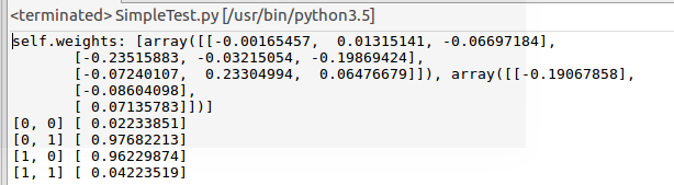
from SimplyNeuralNetwork import NeuralNetwork
import numpy as np
  
nn = NeuralNetwork([2,2,1],'tanh')
  
# 验证异或逻辑
x = np.array([[0,0],[0,1],[1,0],[1,1]])
y = np.array([0,1,1,0])
nn.fit(x,y)
for i in [0,0],[0,1],[1,0],[1,1]:
    print(i,nn.predict(i))

 　　如下倒数4行为预测结果，根据异或运算，和实际结果一致：

六、利用神经网络进行0-9数字预测

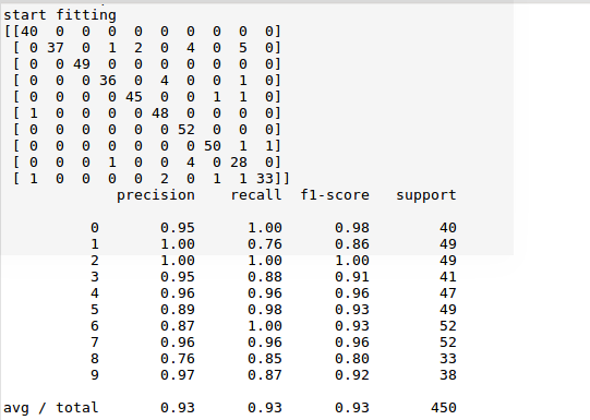
import numpy as np
from sklearn.datasets import load_digits
from sklearn.metrics import confusion_matrix,classification_report
from sklearn.preprocessing import LabelBinarizer
from SimplyNeuralNetwork import NeuralNetwork
from sklearn.cross_validation import train_test_split

digits = load_digits()
X = digits.data
y = digits.target

# 将测试样本值转换为0-1之间的值
X -=X.min()
X /= X.max()

nn = NeuralNetwork([64,100,10],'logistic')
X_train,X_test,y_train,y_test = train_test_split(X,y)
labels_train = LabelBinarizer().fit_transform(y_train)
print(y_train)
print(labels_train)
labels_test = LabelBinarizer().fit_transform(y_test)
print("start fitting")

nn.fit(X_train,labels_train,epochs = 3000)
predictions = []

for i in range(X_test.shape[0]):
    o = nn.predict(X_test[i])
    predictions.append(np.argmax(o))

print(confusion_matrix(y_test,predictions))
print(classification_report(y_test, predictions))

 　　如下对角线表示预测成功的记录数，最下方表示预测成功率统计数据，数据显示，成功率93%，预测效果已经很好：