
基于数据形式说明杜兰特的技术特点的分析(含Python实现讲解部分)
---恢复内容开始---
注: 本博文系原创,转载请标明原处。
题外话:春节过后,回到学校无所事事,感觉整个人都生锈一般,没什么动力,姑且称为“春节后遗症”。在科赛官网得到关于NBA的详细数据,而且又想对于自己学习数据挖掘半年以来做一次系统性梳理,就打算做一份关于杜兰特的技术特点的数据分析报告(本人是杜迷),可以称得上寓学于乐吧。话不多说,开工。。。。。
1 杜兰特 VS Who?
既然要说杜兰特的技术特点,总是要对比吧,不然怎么知道他的特点呢?这里我主要是从几个方面选择:一、球员的位置小前锋和后卫,杜兰特是小前锋,当然也会打打后卫。二、基本是同一个时代的球员,前后差几年也是可以的(如科比)。三、可以称为巨星的球员。最终选择了以下几名球员作为对比:科比、詹姆斯、库里、威斯布鲁克、乔治、安东尼、哈登、保罗、伦纳德。对于新星和前辈们就不做对比,时代不一样数据的意义也有差别,新星的数据比较少,对比没有必要。当然选的人也不是很完美,个人主观选择(哈哈......)
2 数据
数据来源:https://www.kesci.com/apps/home/dataset/599a6e66c8d2787da4d1e21d/document
3 杀向数据的第一刀
巨星表演最佳舞台是季后赛,他们给予我们太多太多的经典时刻,而那些被我们所津津称道时刻就是他们荣誉加身的时刻。所以我打算从季后赛开始分析。。。(就是这么任性)
3.1 首先,我们先看看季后赛的数据有哪些
>>> import pandas as pd
data
>>> data_player_playoff = pd.read_csv('E:\Python\Program\NBA_Data\data\player_playoff.csv')
>>> data_player_playoff.head()
                球员     赛季   球队 结果             比分  时间     投篮  命中  出手   三分 ...  \
0  Kelenna Azubuike  11-12  DAL  L    OKC95-79DAL   5  0.333   1   3  1.0 ...
1  Kelenna Azubuike  06-07  GSW  L  UTA115-101GSW   1    NaN   0   0  NaN ...
2  Kelenna Azubuike  06-07  GSW  W  UTA105-125GSW   3  0.000   0   1  NaN ...
3  Kelenna Azubuike  06-07  GSW  W   DAL86-111GSW   2  1.000   1   1  NaN ...
4  Kelenna Azubuike  06-07  GSW  L  DAL118-112GSW   0    NaN   0   0  NaN ...

   罚球出手  篮板  前场  后场  助攻  抢断  盖帽  失误  犯规  得分
0     0   1   1   0   0   1   0   1   0   3
1     0   0   0   0   0   0   0   0   0   0
2     0   0   0   0   0   0   0   0   1   0
3     0   0   0   0   0   0   0   0   0   2
4     0   0   0   0   0   0   0   0   0   0

[5 rows x 24 columns]
pd.head(n) 函数是对数据前n 行输出,默认5行,pd.tail() 对数据后几行的输出。
3.2 数据的基本信息
>>> data_player_playoff.info()
<class 'pandas.core.frame.DataFrame'>
RangeIndex: 49743 entries, 0 to 49742
Data columns (total 24 columns):
球员      49615 non-null object
赛季      49743 non-null object
球队      49743 non-null object
结果      49743 non-null object
比分      49743 non-null object
时间      49743 non-null int64
投篮      45767 non-null float64
命中      49743 non-null int64
出手      49743 non-null int64
三分      24748 non-null float64
三分命中    49743 non-null int64
三分出手    49743 non-null int64
罚球      29751 non-null float64
罚球命中    49743 non-null int64
罚球出手    49743 non-null int64
篮板      49743 non-null int64
前场      49743 non-null int64
后场      49743 non-null int64
助攻      49743 non-null int64
抢断      49743 non-null int64
盖帽      49743 non-null int64
失误      49743 non-null int64
犯规      49743 non-null int64
得分      49743 non-null int64
dtypes: float64(3), int64(16), object(5)
memory usage: 9.1+ MB
3.3 由于中文的列名对后面的数据处理带来麻烦,更改列名
>>> data_player_playoff.columns = ['player','season','team','result','team_score','time','shoot','hit','shot','three_pts','three_pts_hit','three_pts_shot','free_throw','free_throw_hit','free_throw_shot','backboard','front_court','back_court','assists','steals','block_shot','errors','foul','player_score']
3.4 从数据表中选择杜兰特、科比、詹姆斯、库里、威斯布鲁克、乔治、安东尼、哈登、保罗、伦纳德的数据
>>> kd_data_off = data_player_playoff[data_player_playoff .player == 'Kevin Durant']
>>> jh_data_off = data_player_playoff [data_player_playoff .player == 'James Harden']
>>> kb_data_off = data_player_playoff [data_player_playoff .player == 'Kobe Bryant']
>>> lj_data_off = data_player_playoff [data_player_playoff .player == 'LeBron James']
>>> kl_data_off = data_player_playoff [data_player_playoff .player == 'Kawhi Leonard']
>>> sc_data_off = data_player_playoff [data_player_playoff .player == 'Stephen Curry']
>>> rw_data_off = data_player_playoff [data_player_playoff .player == 'Russell Westbrook']
>>> pg_data_off = data_player_playoff [data_player_playoff .player == 'Paul George']
>>> ca_data_off = data_player_playoff [data_player_playoff .player == 'Carmelo Anthony']
>>> cp_data_off = data_player_playoff [data_player_playoff .player == 'Chris Paul']
>>> super_data_off = pd.DataFrame ()
>>> super_data_off = pd.concat([kd_data_off ,kb_data_off ,jh_data_off ,lj_data_off ,sc_data_off ,kl_data_off ,cp_data_off ,rw_data_off ,pg_data_off ,ca_data_off ])
>>> super_data_off .info()
<class 'pandas.core.frame.DataFrame'>
Int64Index: 1087 entries, 9721 to 904
Data columns (total 24 columns):
player             1087 non-null object
season             1087 non-null object
team               1087 non-null object
result             1087 non-null object
team_score         1087 non-null object
time               1087 non-null int64
shoot              1085 non-null float64
hit                1087 non-null int64
shot               1087 non-null int64
three_pts          1059 non-null float64
three_pts_hit      1087 non-null int64
three_pts_shot     1087 non-null int64
free_throw         1015 non-null float64
free_throw_hit     1087 non-null int64
free_throw_shot    1087 non-null int64
backboard          1087 non-null int64
front_court        1087 non-null int64
back_court         1087 non-null int64
assists            1087 non-null int64
steals             1087 non-null int64
block_shot         1087 non-null int64
errors             1087 non-null int64
foul               1087 non-null int64
player_score       1087 non-null int64
dtypes: float64(3), int64(16), object(5)
memory usage: 212.3+ KB
3.5 把这十个人的数据单独存放到一文件里
>>> super_data_off .to_csv('super_star_playoff.csv',index = False )
4 数据分析
4.1 先看看他们参加了多少场季后赛
>>> super_data_off.player.value_counts()
Kobe Bryant          220
LeBron James         217
Kevin Durant         106
James Harden          88
Kawhi Leonard         87
Russell Westbrook     87
Chris Paul            76
Stephen Curry         75
Carmelo Anthony       66
Paul George           65
Name: player, dtype: int64
这里可以看出詹姆斯的年年总决赛的霸气,只比科比少三场,今年就会超过科比了,而且老詹还要进几年总决赛啊。杜兰特的场数和詹姆斯相差比较大的,估计最后和科比的场数差不多。
4.2 简单粗暴,直接看看他们的季后赛的得分
>>> super_data_off.groupby('player').player_score.describe()
                   count       mean        std   min   25%   50%    75%   max
player
Carmelo Anthony     66.0  25.651515   8.471658   2.0  21.0  25.0  31.00  42.0
Chris Paul          76.0  21.434211   7.691269   4.0  16.0  21.5  27.00  35.0
James Harden        88.0  20.681818  10.485398   0.0  13.0  19.0  28.00  45.0
Kawhi Leonard       87.0  16.459770   8.428640   2.0  11.0  16.0  21.00  43.0
Kevin Durant       106.0  28.754717   6.979987  10.0  25.0  29.0  33.75  41.0
Kobe Bryant        220.0  25.636364   9.856715   0.0  20.0  26.0  32.00  50.0
LeBron James       217.0  28.400922   7.826865   7.0  23.0  28.0  33.00  49.0
Paul George         65.0  18.984615   9.299685   2.0  12.0  19.0  26.00  39.0
Russell Westbrook   87.0  25.275862   8.187753   7.0  19.0  26.0  30.00  51.0
Stephen Curry       75.0  26.200000   8.109054   6.0  21.5  26.0  32.50  44.0
从这里可以看出杜兰特是个得分高手,隐隐约约可以看出稳如狗
得分的直方图来了,坐稳
#coding:utf-8

import matplotlib.pyplot as plt
import pandas as pd
# 中文乱码的处理
from pylab import mpl
mpl.rcParams['font.sans-serif'] = ['FangSong'] # 指定默认字体
mpl.rcParams['axes.unicode_minus'] = False # 解决保存图像是负号'-'显示为方块的问题

super_data_off = pd.read_csv('super_star_playoff.csv')
kd_off_score = super_data_off[super_data_off .player == 'Kevin Durant'] .player_score.describe()
super_off_mean_score = super_data_off .groupby('player').mean()['player_score']
labels = [u'场数',u'均分',u'标准差',u'最小值','25%','50%','75%',u'最大值']
print super_off_mean_score .index
super_name = [u'安东尼',u'保罗',u'哈登',u'伦纳德',u'杜兰特',u'科比',u'詹姆斯',u'乔治',u'威少',u'库里']
# 绘图
plt.bar(range(len(super_off_mean_score )),super_off_mean_score ,align = 'center')

plt.ylabel(u'得分')
plt.title(u'巨星季后赛得分数据对比')
#plt.xticks(range(len(labels)),labels)
plt.xticks(range(len(super_off_mean_score )),super_name)
plt.ylim(15,35)
for x,y in enumerate (super_off_mean_score ):
    plt.text (x, y+1, '%s' % round(y, 2) , ha = 'center')
plt.show()
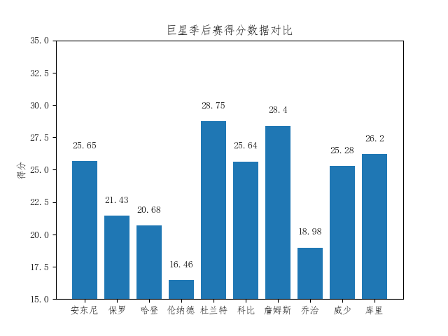
从得分的角度看杜兰特和詹姆斯是一档,安东尼、科比、威少和库里是一档,保罗、哈登、伦纳德、乔治一档。哈登今年应该会有比较明显的提升,毕竟他是从第六人打的季后赛。杜兰特的四个得分王不是白拿的,在得分方面确实联盟的超巨。
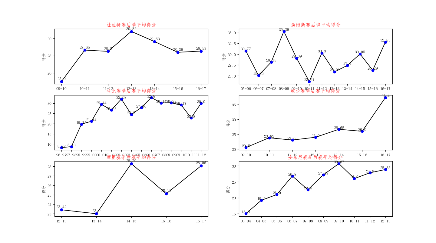
再看看巨星的每个赛季的季后赛的平均值的走势
season_kd_score = super_data_off[super_data_off .player == 'Kevin Durant'] .groupby('season').mean()['player_score']
plt.figure()
plt.subplot(321)
plt.title(u'杜兰特赛后季平均得分',color = 'red')
#plt.xlabel(u'赛季')
plt.ylabel(u'得分')
plt.plot(season_kd_score,'k',season_kd_score,'bo')
for x,y in enumerate (season_kd_score ):
    plt.text (x,y+0.2, '%s' % round(y,2), ha = 'center')


season_lj_score = super_data_off [super_data_off .player == 'LeBron James'].groupby('season').mean()['player_score']
plt.subplot(322)
plt.title(u'詹姆斯赛后季平均得分',color = 'red')
#plt.xlabel(u'赛季')
plt.ylabel(u'得分')
plt.plot(season_lj_score ,'k',season_lj_score ,'bo')
for x,y in enumerate (season_lj_score ):
    plt.text (x,y+0.2, '%s' % round(y,2), ha = 'center')

season_kb_score = super_data_off[super_data_off.player == 'Kobe Bryant'].groupby('season').mean()['player_score']
a = season_kb_score [0:-4]
b =season_kb_score [-4:]
season_kb_score = pd.concat([b,a])
plt.subplot(323)
plt.title(u'科比赛季后赛平均得分',color = 'red')
#plt.xlabel(u'赛季')
plt.ylabel(u'得分')
plt.xticks(range(len(season_kb_score )),season_kb_score.index)
plt.plot(list(season_kb_score) ,'k',list(season_kb_score),'bo')
for x,y in enumerate (season_kb_score ):
    plt.text (x,y+0.2, '%s' % round(y,2), ha = 'center')

season_rw_score = super_data_off[super_data_off.player == 'Russell Westbrook'].groupby('season').mean()['player_score']
plt.subplot(324)
plt.title(u'威少赛季后赛平均得分',color = 'red')
#plt.xlabel(u'赛季')
plt.ylabel(u'得分')
plt.plot(season_rw_score ,'k',season_rw_score ,'bo')
for x,y in enumerate (season_rw_score ):
    plt.text (x,y+0.2, '%s' % round(y,2), ha = 'center')

season_sc_score = super_data_off[super_data_off.player == 'Stephen Curry'].groupby('season').mean()['player_score']
plt.subplot(325)
plt.title(u'库里赛季后赛平均得分',color = 'red')
#plt.xlabel(u'赛季')
plt.ylabel(u'得分')
plt.plot(season_sc_score ,'k',season_sc_score ,'bo')
for x,y in enumerate (season_sc_score ):
    plt.text (x,y+0.2, '%s' % round(y,2), ha = 'center')

season_ca_score = super_data_off[super_data_off.player == 'Carmelo Anthony'].groupby('season').mean()['player_score']
plt.subplot(326)
plt.title(u'安东尼赛季后赛平均得分',color = 'red')
#plt.xlabel(u'赛季')
plt.ylabel(u'得分')
plt.plot(season_ca_score ,'k',season_ca_score ,'bo')
for x,y in enumerate (season_ca_score ):
    plt.text (x,y+0.2, '%s' % round(y,2), ha = 'center')

plt.show()
再使用饼状图观察他们的的得分分布
super_name_E = ['Kevin Durant','LeBron James','Kobe Bryant','Russell Westbrook','Stephen Curry','Carmelo Anthony']
super_name_C = [u'杜兰特',u'詹姆斯',u'科比',u'威少',u'库里',u'安东尼']
plt.figure(facecolor= 'bisque')
colors = ['red', 'yellow', 'peru', 'springgreen']
for i in range(len(super_name_E)):
    player_labels = [u'20分以下',u'20~29分',u'30~39分',u'40分以上']
    explode = [0,0.1,0,0] # 突出得分在20~29的比例
    player_score_range = []
    player_off_score_range = super_data_off[super_data_off .player == super_name_E [i]]
    player_score_range.append(len(player_off_score_range [player_off_score_range['player_score'] < 20])*1.0/len(player_off_score_range ))
    player_score_range.append(len(pd.merge(player_off_score_range[19 < player_off_score_range.player_score],
                                           player_off_score_range[player_off_score_range.player_score < 30],
                                       how='inner')) * 1.0 / len(player_off_score_range))
    player_score_range.append(len(pd.merge(player_off_score_range[29 < player_off_score_range.player_score],
                                           player_off_score_range[player_off_score_range.player_score < 40],
                                       how='inner')) * 1.0 / len(player_off_score_range))
    player_score_range.append(len(player_off_score_range[39 < player_off_score_range.player_score]) * 1.0 / len(player_off_score_range))
    plt.subplot(231 + i)
    plt.title(super_name_C [i] + u'得分分布', color='blue')
    plt.pie(player_score_range, labels=player_labels, colors=colors, labeldistance=1.1,
            autopct='%.01f%%', shadow=False, startangle=90, pctdistance=0.8, explode=explode)
    plt.axis('equal')
plt.show()
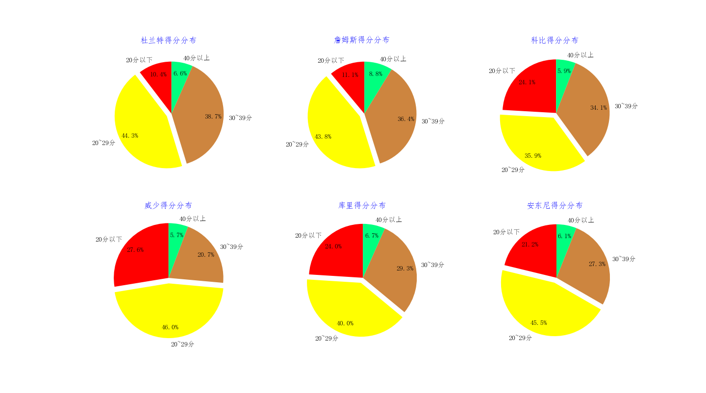
从这些饼状图可知,杜兰特和詹姆斯在得分的稳定性上一骑绝尘,得分主要集中在 20 ~ 40 之间,占到全部的八成左右。他们的不仅得分高,而且稳定性也是极高。其中40+的得分中占比最高的是詹姆斯,其次是库里和杜兰特。这也从侧面得知杜兰特是这些球员中得分最稳的人,真是稳如狗!!!!从数据上看稳定性,那么下面我给出他们的得分的标准差的直方图:
std = super_data_off.groupby('player').std()['player_score']
color = ['red','red','red','red','blue','red','red','red','red','red',]
print std
plt.barh(range(10), std, align = 'center',color = color ,alpha = 0.8)
plt.xlabel(u'标准差',color = 'blue')
plt.ylabel(u'球员', color = 'blue')
plt.yticks(range(len(super_name )),super_name)
plt.xlim(6,11)
for x,y in enumerate (std):
    plt.text(y + 0.1, x, '%s' % round(y,2), va = 'center')
plt.show()
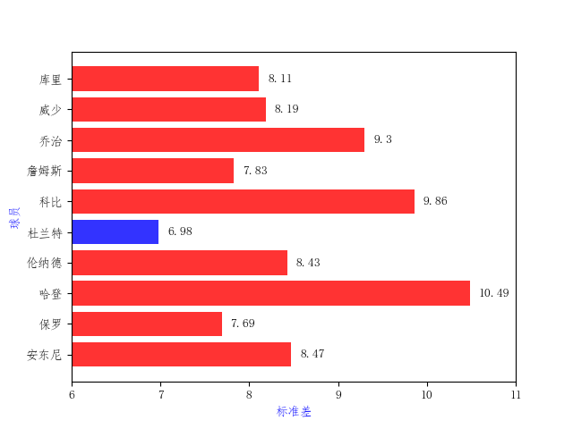
标准差的直方图可以明显地说明杜兰特的稳定性极高(标准差越小说明数据的平稳性越好)
4.3 投篮方式和效率
在评价一个球员时,往往其投篮的区域和命中率是一项很重要的指标,可以把分为神射手,三分投手、中投王和冲击内线(善突),当然也有造犯规的高手,如哈登。
super_name_E = [u'Carmelo Anthony', u'Chris Paul', u'James Harden', u'Kawhi Leonard', u'Kevin Durant', u'Kobe Bryant',
                u'LeBron James', u'Paul George', u'Russell Westbrook', u'Stephen Curry']
bar_width = 0.25
import numpy as np
shoot = super_data_off.groupby('player') .mean()['shoot']
three_pts = super_data_off.groupby('player') .mean()['three_pts']
free_throw = super_data_off.groupby('player') .mean()['free_throw']
plt.bar(np.arange(10),shoot,align = 'center',label = u'投篮命中率',color = 'red',width = bar_width )
plt.bar(np.arange(10)+ bar_width, three_pts ,align = 'center',color = 'blue',label = u'三分命中率',width = bar_width )
plt.bar(np.arange(10)+ 2*bar_width, free_throw  ,align = 'center',color = 'green',label = u'罚球命中率',width = bar_width )
for x,y in enumerate (shoot):
    plt.text(x, y+0.01, '%s' % round(y,2), ha = 'center')
for x,y in enumerate (three_pts ):
    plt.text(x+bar_width , y+0.01, '%s' % round(y,2), ha = 'center')
for x,y in enumerate (free_throw):
    plt.text(x+2*bar_width , y+0.01, '%s' % round(y,2), ha = 'center')
plt.legend ()
plt.ylim(0.3,1.0)
plt.title(u'球员的命中率的对比')
plt.xlabel(u'球员')
plt.xticks(np.arange(10)+bar_width  ,super_name)
plt.ylabel(u'命中率')
plt.show()
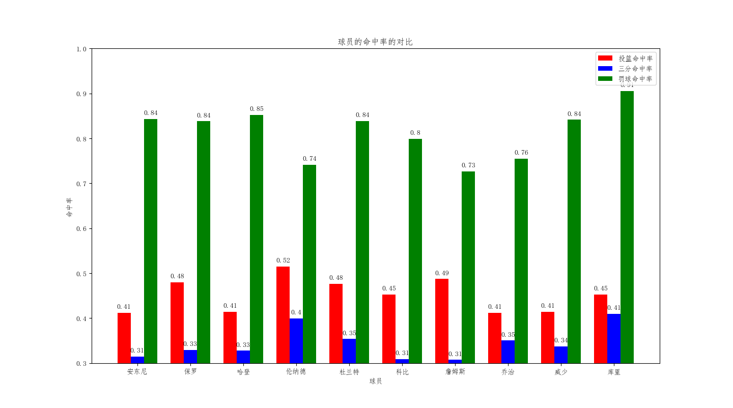
投篮命中率、三分球命中率和罚球命中率最高的依次是伦纳德、库里和库里,由此可见,库里三分能力的强悍。杜兰特这三项的数据都是排在第三位,表明他的得分的全面性。
super_name_E = [u'Carmelo Anthony', u'Chris Paul', u'James Harden', u'Kawhi Leonard', u'Kevin Durant', u'Kobe Bryant',
                u'LeBron James', u'Paul George', u'Russell Westbrook', u'Stephen Curry']
bar_width = 0.25
import numpy as np
three_pts = super_data_off.groupby('player').sum()['three_pts_hit']
free_throw_pts = super_data_off.groupby('player').sum()['free_throw_hit']
sum_pts = super_data_off.groupby('player').sum()['player_score']
three_pts_rate = np.array(list(three_pts ))*3.0 /np.array(list(sum_pts ))
free_throw_pts_rate = np.array(list(free_throw_pts ))*1.0/np.array(list(sum_pts ))
two_pts_rate = 1.0 - three_pts_rate - free_throw_pts_rate
print two_pts_rate
plt.bar(np.arange(10),two_pts_rate ,align = 'center',label = u'二分球得分占比',color = 'red',width = bar_width )
plt.bar(np.arange(10)+ bar_width, three_pts_rate ,align = 'center',color = 'blue',label = u'三分球得分占比',width = bar_width )
plt.bar(np.arange(10)+ 2*bar_width, free_throw_pts_rate   ,align = 'center',color = 'green',label = u'罚球得分占比',width = bar_width )
for x,y in enumerate (two_pts_rate):
    plt.text(x, y+0.01, '%s' % round(y,2), ha = 'center')
for x,y in enumerate (three_pts_rate ):
    plt.text(x+bar_width , y+0.01, '%s' % round(y,2), ha = 'center')
for x,y in enumerate (free_throw_pts_rate):
    plt.text(x+2*bar_width , y+0.01, '%s' % round(y,2), ha = 'center')
plt.legend ()
plt.title(u'球员的得分方式的对比')
plt.xlabel(u'球员')
plt.xticks(np.arange(10)+bar_width  ,super_name)
plt.ylabel(u'占比率')
plt.show()
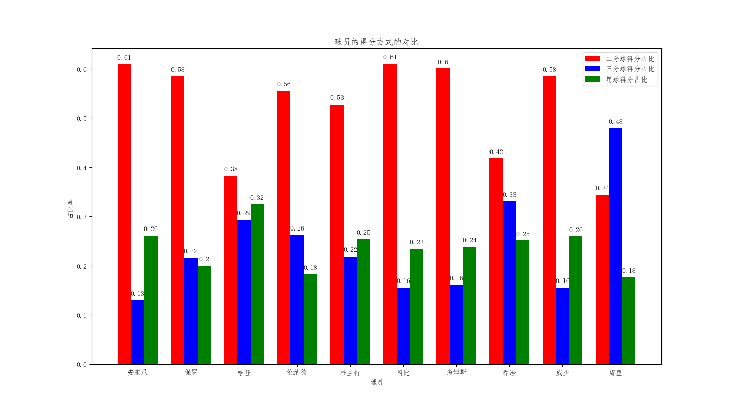
可以看出,二分球占比、三分球占比和罚球占比最高依次是:安东尼和科比、库里 、哈登。这也跟我们的主观相符的,安东尼绝招中距离跳投,科比的后仰跳投,库里不讲理的三分,哈登在罚球的造诣之高,碰瓷王不是白叫的。当然,詹姆斯的二分球占比也是很高,跟他的身体的天赋分不开的。而杜兰特这三项的数据都是中规中矩,也保持着中距离的特点,这也说明了他的进攻的手段的丰富性和全面性。
4.4 防守端的数据
球星的能力不光光体现进攻端,而防守端的能力也是一个重要的指标。强如乔丹、科比和詹姆斯都是最佳防守阵容的常客,所以,这里给出他们在攻防两端的数据值。
import seaborn as sns
import numpy as np
player_adavance = pd.read_csv('super_star_advance_data.csv')
player_labels = [ u'篮板率', u'助攻率', u'抢断率', u'盖帽率',u'失误率', u'使用率', u'胜利贡献值',  u'霍格林效率值']
player_data = player_adavance[['player','total_rebound_rate','assist_rate','steals_rate','cap_rate','error_rate',
                             'usage_rate','ws','per']] .groupby('player').mean()
num = [100,100,100,100,100,100,1,1]
np_num = np.array(player_data)*np.array(num)
plt.title(u'球员攻防两端的能力热力图')
sns.heatmap(np_num , annot=True,xticklabels= player_labels ,yticklabels=super_name  ,cmap='YlGnBu')
plt.show()
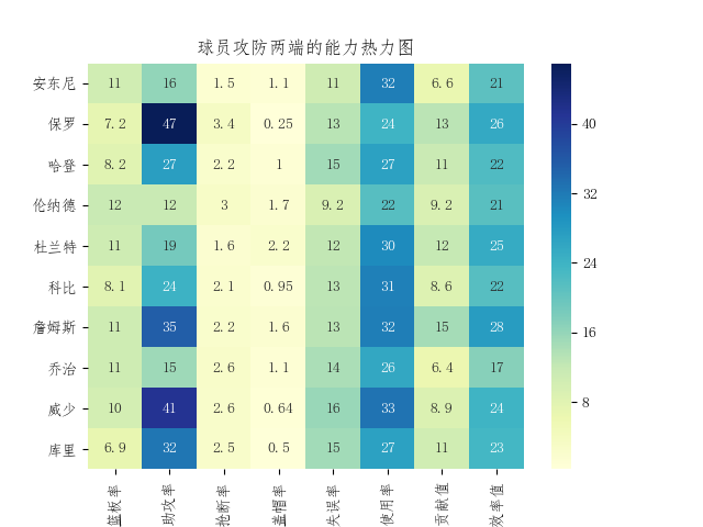
在篮板的数据小前锋的数据差不多,都是11 左右,而后卫中最能抢板是威少,毕竟是上赛季的场均三双(历史第二人)。助攻率最高的当然是保罗,其次是威少和詹姆斯;而杜兰特的助攻率比较平庸,但在小前锋里面也是不错了。抢断率方面是保罗和伦纳德的优势明显,显示了伦纳德的死亡缠绕的效果了。盖帽率最高的是杜兰特,身体的优势在这项数据的体现的很明显;在这个赛季杜兰特的盖帽能力又是提升了一个层次,高居联盟前五(杜中锋,哈哈)。失误率方面后卫高于前锋,最高的是威少。使用率最高的是威少,其次是詹姆斯,可以看出他们的球权都是挺大,伦纳德只有22(波波老爷子的整体篮球控制力真强)。贡献值最高是詹姆斯,毕竟球队都是围绕他建立的,现在更是一个人扛着球队前行;其次是保罗,毕竟球队的大脑;杜兰特第三,也是符合杀神的称号的。效率值的前三和贡献值一样,老詹真是强,不服不行啊。。。。
5 小结
在数据面前,可以得出:从进攻的角度讲,杜兰特是最强的,主要体现在:高得分、稳定性强、得分方式全面和得分效率高。从防守的方面,杜兰特善于封盖,而串联球队方面,杜兰特还是与詹姆斯有着明显差距。这两年杜兰特的防守是越来越好了,希望这个赛季能进入最佳防守阵容。这些数据显示与平时对杜兰特的了解相差不大,可以说数据验证了主观的认识。季后赛的数据就分析就到这里了,对模块padans、numpy 、seaborn 和 matplotlib 系统的梳理一遍吧,也算是新学期的热身吧。常规赛的数据分析就不分析了,什么时候有兴趣了再搞。
---恢复内容结束---

 浙公网安备 33010602011771号