mr 决策树-part1

Part 1: Data | Part 2: Approach | Part 3: Results

-----
Update:  Looks like some folks at Google have built a similar system (albeit much more polished).  You can check it out here.
-----

Recently I've been exploring Hadoop and some of its satellite projects. MapReduce is a powerful paradigm for tackling huge datasets and I wanted a project to help me ease into it all. Mahout, a collection of machine learning algorithms for Hadoop, didn't yet have a C4.5-like implementation for decision trees. C4.5 trees are useful yet conceptually simple, so that seemed like a good place to start.

 

The following few posts will cover my approach toward building a C4.5-like classification tree for Hadoop and follow up with my plans for a regression tree.  This is an educational exercise for me, so if you notice I'm doing something stupid or just have some MapReduce tips or tricks, please let me know!

 

Why do we care?

First things first, why do we care? Why bother with all this Hadoop stuff? How about just sampling a large dataset until the result is small enough for a single machine?

 

For the most part, sampling really is good enough. But if a problem space is extremely complex, then a smaller sample may not give an adequately clear view.

 

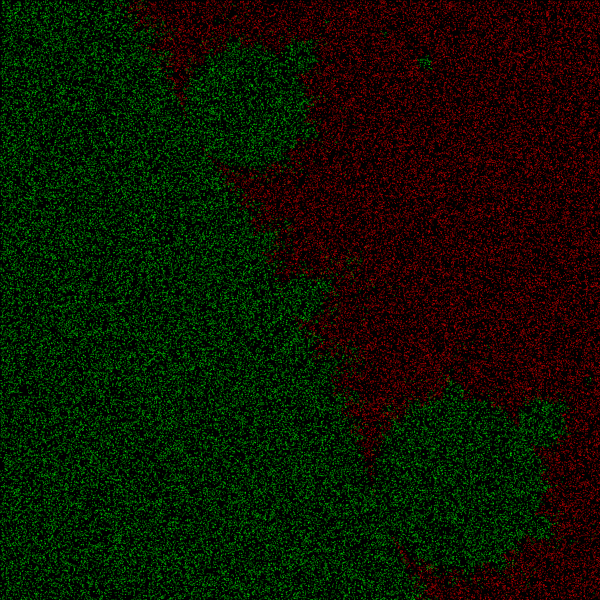
As an example, I've chosen an area of the Mandelbrot set (in Elephant Valley) as my problem space. I choose random points and label them true or false depending on whether they're in the Mandelbrot set or not.

Mandelbrot CSV Sample: 
0.322, 0.093, false
0.301, 0.085, false
0.377, 0.086, true
0.321, 0.089, false

I generated four datasets from this space with sizes of 10 million, 1 million, 100 thousand, and 10 thousand points. I plotted the datasets below by coloring a point red if it's within the Mandelbrot set, green if it is not. As you can see in the plots, 10 million points gives a fairly high fidelity picture of the space. Not surprisingly, 1 million, 100K, and 10K samples give progressively worse detail.  A classifier trained on one of the smaller samples will do well for the majority of space but the lack of resolution near the boundary will make that area troublesome.

Using either Weka's RepTrees (similar to C4.5) or RandomForests, I can learn decision trees for the 10K, 100K, and 1M datasets. The 10M dataset, however, is too large to train the classifiers inside my humble 2GB JVM.

I also generated a second set of data that mirrors the first, but adds 50 dummy features. Each dummy feature is simply a random number between 0 and 1. For this dataset the Weka tree classifiers can only cope with the 10K and 100K samples.

A Hadoop classifier can tackle the larger datasets and, hopefully, produce better results for points in the tricky areas of our problem space. Sampling and using a meta-classifier (like bagging) might do just as well. But, like I said earlier, this is an educational exercise. :)

 

10M Sample

 

1M Sample

 

100K Sample

 

10K Sample

So that's the brief introduction to the data I'll be using in the following posts. Head to the next section to read about the general design for my Hadoop classification tree.

 

Part 1: Data | Part 2: Approach | Part 3: Results

If you're not already familiar with the basics of MapReduce, you may want to check out this tutorial before reading further.

 

The box below shows my shorthand for the four MapReduce tasks that make up the core of the training algorithm. I use parenthesis to wrap key-value pairs. The brackets denote a list.  And I use 'X' when I don't care about the key.

The main departure from the traditional classification tree training process is that we build the tree breadth first instead of depth first. Each iteration of tasks 2 and 3 will grow one layer of the tree.

Task 1:  Initialize the Fields and Tree

Map Input: (X, exampleInstance)

Map Output: (field, fieldValue)

Reduce: (field, fieldDescription)

Create initial tree using the FieldDescriptions

Task 2:  Find Best Split for Each Node-Field Pair

Map Input: (X, exampleInstance)

Map Output: ([leaf, field], [fieldValue, classValue])

Reduce: (X, [leaf, field, fieldSplit,

[informationGain, classCounts],

[informationGain, classCounts]])

Task 3:  Find Best Split for Each Node

Map Input: (X, [leaf, field, fieldSplit,

[informationGain, classCounts],

[informationGain, classCounts]])

Map Output: (leaf, [field, fieldSplit,

[informationGain, classCounts],

[informationGain, classCounts]])

Reduce: (X, [leaf, field, fieldSplit,

[informationGain, classCounts],

[informationGain, classCounts]])

Grow Tree!  Mark any leaves that are finished growing as final.

Repeat tasks 2 and 3 until tree is fully grown.  Optionally include task 4 in the loop.

Task 4:  Prune Instances (remove example instances from final leaves)

Map Input: (X, exampleInstance)

Map Output: (X, exampleInstance)

 - Only output the example if it doesn’t evaluate to a leaf node

Reduce: Identity

Task 1: Initialize Fields and Tree

The first task scans over the input dataset (for now only CSV is supported) to determine whether each field is categorical or numeric. For each categorical field it builds a frequency count over the possible categories. For numeric fields it finds the minimum and maximum values.

The map function for the first task will iterate over the fields of an example instance and output the field id and its value as the key-value pair.

For the Mandelbrot data introduced in the last post there are three fields.  The first two are numeric and the third is categorical; "true" or "false". Below is the map output for a few example points.

Map Input -> Map Output
(X, [0.322, 0.093, false])
 -> (0, 0.322), (1, 0.093), (2, false)

(X, [0.301, 0.085, false])
 -> (0, 0.301), (1, 0.085), (2, false)
(X, [0.377, 0.086, true])
 -> (0, 0.377), (1, 0.086), (2, true) 
(X, [0.321, 0.089, false])
 -> (0, 0.321), (1, 0.089), (2, false)

Since we used the field id as a key, the reduce function iterates over all the values for a field. For now, I assume that categorical fields will never have values parsable as a number (things like zipcode would break this assumption). It's restrictive but it makes it easy to discriminate between data types. I'll mention a better way to determine type in a later post.

 

Reduce Input -> Reduce Output
(0, [0.322, 0.301, 0.377, 0.321])
 -> [numeric, min:0.301, max:0.377]
(1, [0.093, 0.085, 0.086, 0.089])
 -> [numeric, min:0.085, max:0.093]
(2, [false, false, true, false])
 -> [categorical, false:3, true:1]

We now have field descriptions for our training dataset.  Also, we require the index of the objective class field as a parameter when running this algorithm.  With the class field and the field descriptions, we have enough information to create a classification tree.  At this point, it's nothing more than a root node.  But it's a start.

 

I have a home-cooked XML format for classification trees. Ideally I'd use something like PMML, but for now that's still on the to-do list. Anyway, here is the simple tree for our four examples after task 1 completes:

 

<tree objectiveFieldIndex="2">
  <fields>
    <field index="0" isCategorical="false" min="0.301" max="0.377"/>
    <field index="1" isCategorical="false" min="0.085" max="0.093"/>
    <field index="2" isCategorical="true">
      <category value="false" count="3"/>
      <category value="true" count="1"/>
    </field>
  </fields>
  <root id="0" isLeaf="false">
    <classCounts>
      <classCount classCategory="false" count="3"/>
      <classCount classCategory="true" count="1"/>
    </classCounts>
  </root>
</tree>

Task 2: Find Best Split for Each Node-Field Pair

This MapReduce task is core for the entire process. It does the majority of the work to find out which splitting conditions we should use to further grow the tree. But before it starts we need to use one of Hadoop's essential features, the distributed cache. We use the distributed cache to share our tree's XML file with the machines that will be processing task 2.

 

Each map node will load our tree into memory before it starts working. Like task 1, every training example from our dataset will be mapped. The map method evaluates the training example on the classification tree to find which leaf node the example 'falls' into.  For each field (excepting the class field), the map method will output a key composed of the id of the leaf node and the field id.  The output value consists of the field's value and the class field's value.

 

For our little example, the tree's root node has a node id of 0.  As you'd expect, all four of the training instances evaluate to the root node since it has no children.

 

Map Input -> Map Output

 

(X, [0.322, 0.093, false])
 -> ([0, 0], [0.322, false]), ([0, 1], [0.093, false])

(X, [0.301, 0.085, false])
 -> ([0, 0], [0.301, false]), ([0, 1], [0.085, false])

(X, [0.377, 0.086, true])
 -> ([0, 0], [0.377, true]), ([0, 1], [0.086, true])

(X, [0.321, 0.089, false])
 -> ([0, 0], [0.321, false]), ([0, 1], [0.089, false])

 

The reduce step will iterate over all the values for each node-field pair. During this task we're looking to find the best split possible given a field and a tree leaf node. To do this, during our iteration we maintain class category frequency counts for all candidate splits. After we've gathered the class frequency counts we can compute which split has the highest information gain.

 

To maintain the counts for each split we must first determine the set of possible splits. To keep it simple, we only consider binary splits. For a categorical field there will be a candidate split for each possible category (field == someCategory).

 

For a numeric fields the set of candidate splits are a little more tricky (field <= someNumber). The original C4.5 formulation suggested testing a split between each adjacent pair of field values. This, however, doesn't scale so nicely to 'big data' problems. If we're running on a dataset with 10 million points we could end up testing 10 million possible splits for each numeric field. No good.

 

So for this algorithm, we instead use a fixed number of split candidates. I normally use 10000 split candidates, but any value should work as long as there's memory enough to maintain that many separate class frequency counts. We evenly divide a numeric field's range into 'splitCandidates+1' buckets. The possible split values are the thresholds between the buckets. Now while the reducer iterates, we just maintain the class frequency count for each bucket and we have the information needed to find the best split point.

 

For our little example, I used 2 split candidates for numeric fields. That means we'll divide a numeric field's range into 3 buckets.  Field 0 has a range of 0.301 to 0.377. So each bucket will be 0.025 wide and our split candidate points will be at 0.326 and 0.351. The reducer can now count up class frequencies and find the best split point for the feature. The final output for the reducing step will look something like:

 

Reduce Input -> Reduce Output

 

([0, 0], [[0.322, false], [0.301, false],
          [0.377, true], [0.321, false]])
 -> (X, [0, 0, <= 0.326, 0.811, [false:3, true:0], [false:0, true:1]])

 

([0, 1], [[0.093, false], [0.085, false],
          [0.086, true], [0.089, false]])
 -> (X, [0, 1, <= 0.0877, 0.311, [false:1, true:1], [false:2, true:0]])

Task 3: Find Best Split for Each Node

For each leaf node, task 2 will produce the best split for each field.  Task 3 will narrow this down by choosing the single best split for each leaf node. 

 

The MapReduce steps in this task are straight forward. The map method takes the output task 2 and simply pulls the leaf id out of the value and makes it the key.

 

Map Input -> Map Output

 

(X, [0, 0, <= 0.326, 0.811, [false:3, true:0], [false:0, true:1]])

 -> (0, [0, <= 0.326, 0.811, [false:3, true:0], [false:0, true:1])

 

(X, [0, 1, <= 0.0877, 0.311, [false:1, true:1], [false:2, true:0]])

 -> (0, [1, <= 0.0877, 0.311, [false:1, true:1], [false:2, true:0]])

The reduce step will iterate over all the candidate splits for a leaf node and simply output the one with the maximum information gain.

 

Reduce Input -> Reduce Output

(0, [[0, <= 0.326, 0.811, [false:3, true:0], [false:0, true:1],

     [0, 1, <= 0.0877, 0.311, [false:1, true:1], [false:2, true:0]])

 -> (0, [0, <= 0.326, 0.811, [false:3, true:0], [false:0, true:1])

 

The reducer output gives us the information we need to grow the next generation of the tree. We iterate steps 2 and 3 until the tree is fully grown. And there we have a basic algorithm for growing a classification tree on "big data". I'll cover some caveats and possible improvements to this approach in the next section.

Continue to Part 3: Results.

 

Decision Trees & Hadoop - Part 3: Results

 

Part 1: Data | Part 2: Approach | Part 3: Results

And now the (exciting?) conclusion of my adventures building a C4.5-like decision tree with Hadoop. Since my previous post I've implemented the design, added a few new wrinkles, and collected the results using my Mandelbrot toy problem.

 

I'm skipping the low level details, but the "new wrinkles" are two additional map-reduce tasks.

 

One of the tasks triggers whenever the number of instances in a tree node drops below a predefined threshold. The threshold is set low enough that we know the instances can fit into the processes' memory. So we go ahead and grow the rest of that tree branch in the standard recursive manner, greatly reducing the time it takes to build the entire tree.

 

The second task simply searches for instances that belong to leaves of the tree (nodes we no longer consider for splitting) and removes them. This reduces the amount of data we need to evaluate in future iterations.

 

I ran the Hadoop tree algorithm on the toy dataset I described in part 1 and compared it to the RepTree and RandomForest techniques from Weka's collection. RepTree and the RandomForest outperformed HadoopTree for 10K, 100K, and 1M datasets, but failed to build on the 10M dataset (using a 2 GB JVM). The HadoopTree trained on the 10M dataset had the best overall accuracy.

 

To give the HadoopTree fair competition I added 11 bagged RepTrees (bagging being a more traditional way to tackle giant datasets). The bagged RepTree's performance was nearly an exact match of the HadoopTree's results.

 

In the second round of tests I used Mandelbrot data with 50 dummy numeric features. This made the dataset much larger and RepTree and RandomForest failed to build on both the 1M and 10M datasets. Random splits don't do well with a large number of junk features so, not surprisingly, the RandomForest's performance suffered on this dataset.

 

The HadoopTree trained on 10M instances carries the day, but a bag of 101 RepTrees comes in a close second. Considering that bagged smaller trees are much faster to grow and would do better on noisy data, the single HadoopTree is more novelty than practical. Although I'm not implementing it at the moment, I expect this technique would provide a bigger payoff if it were modified to grow boosted regression trees.

See the full results here.

The code is viewable on GitHub, but be warned, it's still a toy project. I haven't serialized the output from the map-reduce tasks (so there's a lot more data transfer than there should be) or made a proper parameter/config file.