四、神经网络（深度学习算法）

4.1 认识神经网络

• 必要性
  • 当特征值只有两个时，我们仍可以用之前学过的算法去解决
  • 
  • 但当特征值很多，且含有很多个多次多项式时，用之前的算法就很难解决了
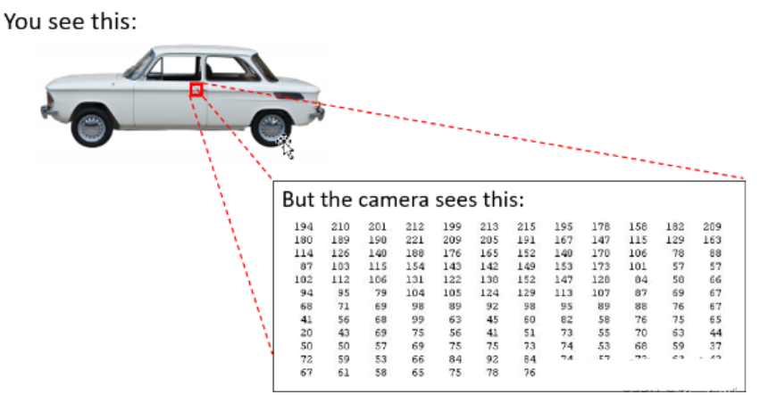
    例子 ：图像感知 Recogonition image
    计算机识别汽车是靠像素点的亮度值
  •   

神经网络做法：

4.2 如何在神经网络上推理

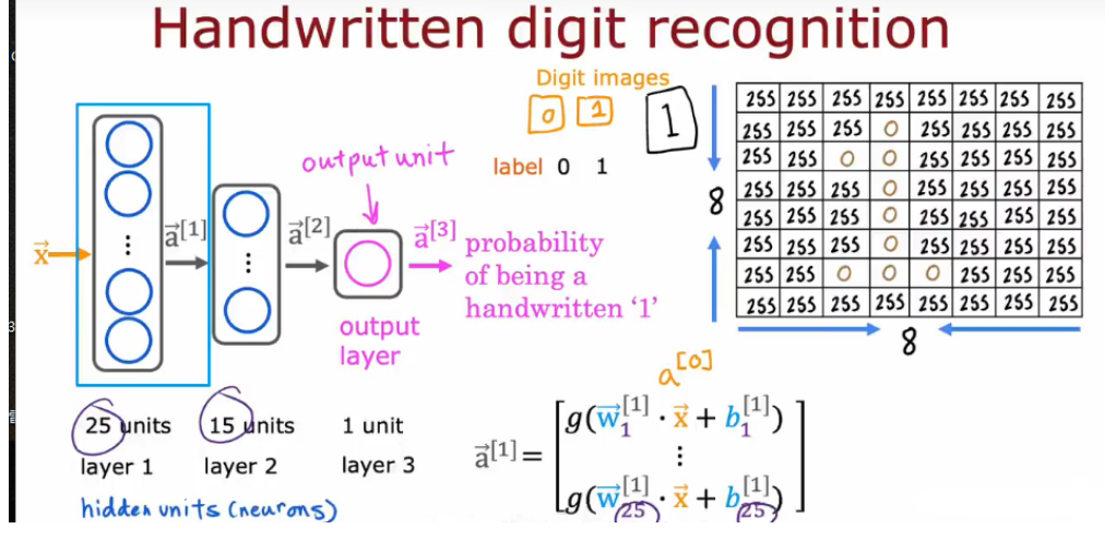
4.2.1 神经网络定义

定义一个神经网络如下：

计算第l层第j个激活值的公式：

注意符号的含义 w2_1 上标2代表layer 2 下标 1代表第一个神经元

4.2.2 构建：前向传播 forward propagation（使用TensorFlow实现）

前向传播是从输入层开始，通过各层计算直至输出层，从而得出预测结果。

• eg1：手写识别0、1
  •   
  • 每次层计算， 从左往右计算，要传播神经元的激活值
  • 
• eg2：烤咖啡的好坏
  • 
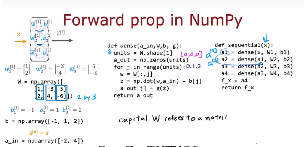
  • python实现前向传播
  • 
  • 自定义dense密集函数：输入前一层的激活，给定当前层的参数，它会输出下一层激活值 自定义sequential函数
其中：W大写在线性代数中代表矩阵
• 拓展： AGI 通用人工智能
  • 

4.3 课后作业

import numpy as np
import matplotlib.pyplot as plt
import pandas as pd
from scipy.io import loadmat
from scipy.optimize import minimize

# 加载数据集，这里的数据为matlab格式，所有要用SciPy.io的loadmat函数
def load_data(path):
    data = loadmat(path)
    X = data['X']
    y = data['y']
    return X, y

X, y = load_data('ex3data1.mat')
print(np.unique(y))  # 找到数组 y 中的所有唯一元素，并返回一个已排序的数组
# [ 1  2  3  4  5  6  7  8  9 10]
X.shape, y.shape
# ((5000, 400), (5000, 1))
# 其中有5000个训练样本，每个样本是20 * 20
# 像素的数字的灰度图像。每个像素代表一个浮点数，表示该位置的灰度强度。20×20的像素网格被展开成一个400维的向量。
# 在我们的数据矩阵X中，每一个样本都变成了一行，这给了我们一个5000×400矩阵X，每一行都是一个手写数字图像的训练样本。

# 第一个任务是将我们的逻辑回归实现修改为完全向量化（即没有“for”循环）。
# 这是因为向量化代码除了简洁外，还能够利用线性代数优化，并且通常比迭代代码快得多。
# Visualizing the data
def plot_an_image(X):
    """
    随机打印一个数字
    """
    pick_one = np.random.randint(0, 5000)  # 从0到5000中随机选取一个整数
    image = X[pick_one, :]  # 从数据集中选取这个随机索引对应的图像数据
    fig, ax = plt.subplots(figsize=(1, 1))
    # 将选取的图像数据重新塑形为20x20的矩阵，并使用灰度反转的颜色显示
    ax.matshow(image.reshape((20, 20)), cmap='gray_r')  # matshow用于以矩阵形式显示二维数组
    plt.xticks([])
    plt.yticks([])  # 去除x轴和y轴的刻度，使图像显示更美观。
    plt.show()
    print('this should be {}'.format(y[pick_one]))

def plot_100_image(X):
    """
    随机画100个数字
    """
    sample_idx = np.random.choice(np.arange(X.shape[0]), 100)
    sample_images = X[sample_idx, :]  # (100, 400)
    # 创建一个10x10的子图网格，共享x轴和y轴的刻度和标签，图像大小为8x8英寸
    fig, ax_array = plt.subplots(nrows=10, ncols=10, sharey=True, sharex=True, figsize=(8, 8))
    for row in range(10):
        for column in range(10):
            ax_array[row, column].matshow(sample_images[10 * row + column].reshape((20, 20)), cmap='gray_r')
    plt.xticks([])
    plt.yticks([])
    plt.show()

# Vectorizing Logistic Regression
    # 我们将使用多个one-vs-all(一对多)logistic回归模型来构建一个多类分类器。由于有10个类，需要训练10个独立的分类器。
    # 为了提高训练效率，重要的是向量化。
# Vectorizing the cost function
def sigmoid(z):
    return 1 / (1 + np.exp(-z))

def regularized_cost(theta, X, y, l):
    """
        don't penalize theta_0
        args:
            X: feature matrix, (m, n+1) # 插入了x0=1
            y: target vector, (m, )
            l(正则化常数λ): lambda constant for regularization
    """
    thetaReg = theta[1:]
    first = (-y*np.log(sigmoid(X@theta))) + (y-1)*np.log(1-sigmoid(X@theta))
    reg = (thetaReg@thetaReg)*l / (2*len(X))
    return np.mean(first) + reg

# Vectorizing the gradient
def regularized_gradient(theta, X, y, l):
    """
        don't penalize theta_0
        args:
            l: lambda constant
        return:
            a vector of gradient
    """
    thetaReg = theta[1:]
    first = (1 / len(X)) * X.T @ (sigmoid(X @ theta) - y)
    # 这里人为插入一维0，使得对theta_0不惩罚，方便计算
    reg = np.concatenate([np.array([0]), (l / len(X)) * thetaReg])  # 使用np.concatenate将上面两个数组连接在一起。
    return first + reg

# One-vs-all Classification
# 这部分我们将实现一对多分类通过训练多个正则化logistic回归分类器，每个对应数据集中K类中的一个。
# 对于这个任务，我们有10个可能的类，并且由于logistic回归只能一次在2个类之间进行分类，每个分类器在“类别i”和“不是i”之间决定。
# 我们将把分类器训练包含在一个函数中，该函数计算10个分类器中的每个分类器的最终权重，并将权重返回shape为(k,(n + 1))数组，其中n是参数数量。
def one_vs_all(X, y, l, K):
    """generalized logistic regression
        args:
            X: feature matrix, (m, n+1) # with incercept x0=1
            y: target vector, (m, )
            l: lambda constant for regularization λ控制正则化强度
            K: numbel of labels
        return: trained parameters
    """
    all_theta = np.zeros((K, X.shape[1]))  # (10, 401)
    for i in range(1, K+1):
        theta = np.zeros(X.shape[1])
        y_i = np.array([1 if label == i else 0 for label in y])

        ret = minimize(fun=regularized_cost, x0=theta, args=(X, y_i, l), method='TNC',
                       jac=regularized_gradient, options={'disp': True})  # 设置disp为True以显示优化过程。
        all_theta[i - 1, :] = ret.x
    return all_theta


# 这里需要注意的几点：首先，我们为X添加了一列常数项1 ，以计算截距项（常数项）。
# 其次，我们将y从类标签转换为每个分类器的二进制值（要么是类i，要么不是类i）。 最后，我们使用SciPy的较新优化API来最小化每个分类器的代价函数。
# 如果指定的话，API将采用目标函数，初始参数集，优化方法和jacobian（渐变）函数。 然后将优化程序找到的参数分配给参数数组。

# 实现向量化代码的一个更具挑战性的部分是正确地写入所有的矩阵，保证维度正确。
def predict_all(X, all_theta):
    # 计算每个样本在每个类别上的概率
    h = sigmoid(X @ all_theta.T)  # 注意的这里的all_theta需要转置
    # 创建一个数组，包含每个样本概率最大的类别的索引
    # axis=1,返回沿着每行或水平方向最大值的索引
    h_argmax = np.argmax(h, axis=1)
    # 将索引值从0开始的数组转换为从1开始的数组。
    h_argmax = h_argmax + 1
    return h_argmax
# 这里的h共5000行，10列，每行代表一个样本，每列是预测对应数字的概率。我们取概率最大对应的index加1就是我们分类器最终预测出来的类别。
# 返回的h_argmax是一个array，包含5000个样本对应的预测值。
raw_X, raw_y = load_data('ex3data1.mat')
X = np.insert(raw_X, 0, 1, axis=1)  # (5000, 401)
y = raw_y.flatten()  # 这里消除了一个维度，将其转换为一维数组，方便后面的计算 or .reshape(-1) （5000，）

all_theta = one_vs_all(X, y, 1, 10)
all_theta  # 每一行是一个分类器的一组参数
y_pred = predict_all(X, all_theta)
accuracy = np.mean(y_pred == y)
print('accuracy = {0}%'.format(accuracy * 100))

# Neural Networks
# 上面使用了多类logistic回归，然而logistic回归不能形成更复杂的假设，因为它只是一个线性分类器。
# 接下来我们用神经网络来尝试下，神经网络可以实现非常复杂的非线性的模型。我们将利用已经训练好了的权重进行预测。
def load_weight(path):
    data = loadmat(path)
    return data['Theta1'], data['Theta2']

theta1, theta2 = load_weight('ex3weights.mat')
# theta1.shape, theta2.shape
# 因此在数据加载函数中，原始数据做了转置，然而，转置的数据与给定的参数不兼容，因为这些参数是由原始数据训练的。
# 所以为了应用给定的参数，需要使用原始数据（不转置）
X, y = load_data('ex3data1.mat')
y = y.flatten()
# 向特征矩阵 X 的每一行开头插入一个值为1的列
X = np.insert(X, 0, values=np.ones(X.shape[0]), axis=1)
X.shape, y.shape

a1 = X
z2 = a1 @ theta1.T
# z2.shape
z2 = np.insert(z2, 0, 1, axis=1)
a2 = sigmoid(z2)
# a2.shape
z3 = a2 @ theta2.T
# z3.shape
a3 = sigmoid(z3)
# a3.shape
y_pred = np.argmax(a3, axis=1) + 1
accuracy = np.mean(y_pred == y)
print ('accuracy = {0}%'.format(accuracy * 100))  # accuracy = 97.52%

4.4 训练神经网络

4.4.1 模型训练细节

• eg：对于01手写分类问题
  • 
  • 对于逻辑回归、二分类问题用Binary Cross Entropy二元交叉熵损失函数
  • 
  • 使用二元交叉熵作为损失函数时，我们通常使用以下公式来计算单个样本的损失：
  • loss = -[ylog(p) + (1-y)log[(1-p)]
  • 其中，y是真实标签（0或1），p是预测值（0到之间的概率值）。这个公式表示当真实标签为1时，我们希望预测值越接近1，此时损失越小，等于-log(p);
  • 当真实标签为0时，我们希望预测值p越接近0，此时损失也越小，等于-log(1-p)。
  • 

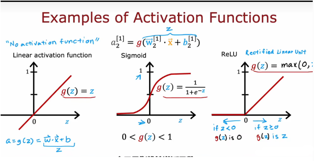
4.4.2 如何选择激活函数

• 三种基础激活函数
  • 
• 对于输出层激活函数的选择，取决于输出的y的取值范围
  • 
• hidden layer 隐藏层
  • 除非是二分类问题用sigmoid，一般默认用relu，不能用线性激活函数，否则不能拟合，就相当于一个线性回归了
  • relu计算很快，并且只有右边扁平flat，而sigmoid有两处flat，会影响gd的速度

4.5 多分类问题

4.5.1 softmax 回归算法

• Softmax 回归（Softmax Regression）是一种广义的逻辑回归，用于多分类问题。它可以看作是二分类逻辑回归的扩展，能够同时处理多个类别。Softmax 回归通常用于神经网络的输出层，将输出值转换为概率分布。
• Softmax 回归算法的模型（参考）
  • 
  • 
• 输出层计算方式
  • 
  • 输出层也叫作softmax层，输出的K维向量a，中的每一个分量都与z1-z10有关系，这个和之前学的不太一样

4.5.2 多标签分类问题

输出值y是一个向量，而不是一个数，不能用softmax，因为比如既有人又有车（每个样本可以有多个类别标签）无法处理，对每个分量用sigmoid

4.6 高级优化方法

4.6.1 Adam 算法 自适应距估计 ——自动调节学习率大小

需要一个默认的学习率，建议可以选一个大点，一个小点的多试

4.7 其他网络层的类型

• dense layer 密集层就是全连接层一种隐藏层，其中的每个节点均与下一个隐藏层中的每个节点相连。
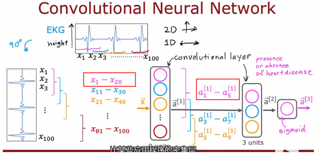
• convolutional layer 卷积层
  例子：心电图识别，判断是否有心脏病，二分类
  • 
  • 需要考虑的参数：
单个神经元应该观 察的输入窗口有多大？
一层应该有几个神经元？

4.8 课后习题

import numpy as np
import matplotlib.pyplot as plt
from scipy.io import loadmat
import scipy.optimize as opt
from sklearn.metrics import classification_report

# Visualizing the data 可视化数据
def load_mat(path):
    """读取数据"""
    data = loadmat('ex4data1.mat')
    X = data['X']
    Y = data['y'].flatten()
    return X, Y

def plot_100_images(X):
    """随机画100个数字"""
    index = np.random.choice(range(5000), 100)
    images = X[index]
    # fig, ax_array创建多个子图
    fig, ax_array = plt.subplots(10, 10, sharey=True, sharex=True, figsize=(8, 8))
    for r in range(10):
        for c in range(10):
            ax_array[r, c].matshow(images[r*10 + c].reshape(20, 20), cmap='gray_r')
    plt.xticks([])
    plt.yticks([])
    plt.show()

X, y = load_mat('ex4data1.mat')
plot_100_images(X)

# Model representation 模型表示
#     我们的网络有三层，输入层，隐藏层，输出层。我们的输入是数字图像的像素值，因为每个数字的图像大小为20*20，
#     所以我们输入层有400个单元（这里只考虑图像的像素值，不包括偏置单元。）。
#     在神经网络中，偏置单元（bias unit）是一个额外的节点，通常用于增加模型的灵活性和提高拟合数据的能力。
#     偏置单元在每一层的输出中增加一个恒定的值（通常是1），这允许神经网络在没有输入特征值的情况下也能够进行输出。
# load train data set 读取数据
#     首先我们要将标签值（1，2，3，4，…，10）转化成非线性相关的向量，向量对应位置（y[i-1]）上的值等于1，
#     例如y[0]=6转化为y[0]=[0,0,0,0,0,1,0,0,0,0]。
from sklearn.preprocessing import OneHotEncoder
def expand_y(y):
    result = []
    # 把y中每个类别转化为一个向量，对应的lable值在向量对应位置上置为1
    for i in y:
        y_array = np.zeros(10)
        y_array[i-1] = 1
        result.append(y_array)
        '''
            # 或者用sklearn中OneHotEncoder函数
            encoder =  OneHotEncoder(sparse=False)  # return a array instead of matrix
            y_onehot = encoder.fit_transform(y.reshape(-1,1))
            return y_onehot
        '''
    return np.array(result)  # 将 result 转换为 NumPy 数组
# 获取训练数据集，以及对训练集做相应的处理，得到我们的input X，lables y。
raw_X, raw_y = load_mat('ex4data1.mat')
X = np.insert(raw_X, 0, 1, axis=1)
y = expand_y(raw_y)
X.shape, y.shape  # ((5000, 401), (5000, 10))
# load weight 读取权重
#     这里我们提供了已经训练好的参数θ1，θ2，存储在ex4weight.mat文件中。
#     这些参数的维度由神经网络的大小决定，第二层有25个单元，输出层有10个单元(对应10个数字类)。
def load_weight(path):
    data = loadmat(path)
    return data['Theta1'], data['Theta2']
t1, t2 = load_weight('ex4weights.mat')
t1.shape, t2.shape  # ((25, 401), (10, 26))
# 展开参数
#     当我们使用高级优化方法来优化神经网络时，我们需要将多个参数矩阵展开，才能传入优化函数，然后再恢复形状。
def serialize(a, b):
    '''展开参数'''
    return np.r_[a.flaten(), b.flaten()]  # 将两个数组 a 和 b 展平为一维数组后按行连接起来，形成一个新的一维数组。
theta = serialize(t1, t2)  # 扁平化参数，25*401+10*26=10285
theta.shape  # (10285,)
def deserialize(seq):
    '''从 seq 中提取前 25*401 个元素。这些元素被认为是输入层到隐藏层的权重。再提取剩余的元素，这些元素被认为是隐藏层到输出层的权重。'''
    return seq[:25*401].reshape(250, 401), seq[25*401:].reshape(10, 26)

# Feedforward and cost function 前馈和代价函数
# Feedforward
#     确保每层的单元数，注意输出时加一个偏置单元，s(1)=400+1，s(2)=25+1，s(3)=10。
def sigmoid(z):
    return 1 / (1 + np.exp(-z))
def feed_forward(theta, X):
    '''得到每层的输入和输出'''
    t1 , t2 = deserialize(theta)
    # 前面已经插入过偏置单元，这里就不用插入了
    a1 = X
    z2 = a1 @ t1.T
    a2 = np.insert(sigmoid(z2), 0, 1, axis=1)
    z3 = a2 @ t2.T
    a3 = sigmoid(z3)
    return a1, z2, a2, z3, a3
a1, z2 , a2, z3, h = feed_forward(theta, X)
# Cost function
#     输出层输出的是对样本的预测，包含5000个数据，每个数据对应了一个包含10个元素的向量，代表了结果有10类。
#     在公式中，每个元素与log项对应相乘。最后我们使用提供训练好的参数θ，算出的cost应该为0.287629
def cost(theta, X, y):
    # 进行前向传播计算，获取神经网络每一层的激活值和最终的预测值
    a1, z2 , a2, z3, a3, h = feed_forward(theta, X)
    J = 0
    J = - y * np.log(h) - (1 - y) * np.log(1 - h)
    return J.sum() / len(X)
cost(theta, X, y)

# Regularized cost function 正则化代价函数
#     注意不要将每层的偏置项正则化
def regularized_cost(theta, X, y, l=1):
    '''正则化时忽略每层的偏置项，也就是参数矩阵的第一列'''
    t1, t2 = deserialize(theta)
    reg = np.sum(t1[:,1:] ** 2) + np.sum(t2[:,1:] ** 2)
    return 1 / (2 * len(X)) * reg + cost(theta, X, y)
regularized_cost(theta, X, y, 1)  # 0.38376985909092354

# Backpropagation 反向传播
# Sigmoid gradient S函数导数
def sigmoid_gradient(z):
    return sigmoid(z) * (1 - sigmoid(z))
# Random initialization 随机初始化
#     当我们训练神经网络时，随机初始化参数是很重要的，可以打破数据的对称性。
#     一个有效的策略是在均匀分布(−e，e)中随机选择值，我们可以选择 e = 0.12 这个范围的值来确保参数足够小，使得训练更有效率。
def random_init(size):
    '''从服从的均匀分布的范围中随机返回size大小的值'''
    return np.random.uniform(-0.12, 0.12, size)
# 反向传播
#     目标：获取整个网络代价函数的梯度。以便在优化算法中求解。
#     这里面一定要理解正向传播和反向传播的过程，才能弄清楚各种参数在网络中的维度，切记。比如手写出每次传播的式子。
print('a1', a1.shape,'t1', t1.shape)
print('z2', z2.shape)
print('a2', a2.shape, 't2', t2.shape)
print('z3', z3.shape)
print('a3', h.shape)
'''
a1 (5000, 401) t1 (25, 401)
z2 (5000, 25)
a2 (5000, 26) t2 (10, 26)
z3 (5000, 10)
a3 (5000, 10)
'''
def gradient(theta, X, y):
    '''
    unregularized gradient, notice no d1 since the input layer has no error
    return 所有参数theta的梯度，故梯度D(i)和参数theta(i)同shape，重要。
    '''
    # 反序列化theta，得到t1和t2
    t1, t2 = deserialize(theta)
    # 前向传播计算a1, z2, a2, z3, h
    a1, z2, a2, z3, h = feed_forward(theta, X)
    # 输出层误差计算
    d3 = h - y  # (5000, 10)
    # 隐藏层误差计算（忽略偏置单元）
    d2 = d3 @ t2[:, 1:] * sigmoid_gradient(z2)  # (5000, 25)
    # 计算输出层的梯度
    D2 = d3.T @ a2  # (10, 26)
    # 计算隐藏层的梯度
    D1 = d2.T @ a1  # (25, 401)
    # 序列化梯度，计算平均值
    D = (1 / len(X)) * serialize(D1, D2)  # (10285,)
    return D
# Gradient checking 梯度检测(验证反向传播算法正确性的方法)
#     在你的神经网络,你是最小化代价函数J(Θ)。
#     执行梯度检查你的参数,你可以想象展开参数Θ(1)Θ(2)成一个长向量θ。通过这样做,你能使用以下梯度检查过程。
def gradient_checking(theta, X, y, e):
    def a_numeric_grad(plus, minus):
        """
        对每个参数theta_i计算数值梯度，即理论梯度。
        """
        return (regularized_cost(plus, X, y) - regularized_cost(minus, X, y)) / (e * 2)

    numeric_grad = []
    for i in range(len(theta)):
        plus = theta.copy()  # deep copy otherwise you will change the raw theta
        minus = theta.copy()
        plus[i] = plus[i] + e
        minus[i] = minus[i] - e
        grad_i = a_numeric_grad(plus, minus)
        numeric_grad.append(grad_i)

    numeric_grad = np.array(numeric_grad)
    analytic_grad = regularized_gradient(theta, X, y)
    diff = np.linalg.norm(numeric_grad - analytic_grad) / np.linalg.norm(numeric_grad + analytic_grad)
    # 打印相对差异。如果相对差异小于10的-9次方，说明反向传播实现是正确的。
    print(
        'If your backpropagation implementation is correct,\nthe relative difference will be smaller than 10e-9 (assume epsilon=0.0001).\nRelative Difference: {}\n'.format(
            diff))
gradient_checking(theta, X, y, 0.0001)  #这个运行很慢，谨慎运行
# Regularized Neural Networks 正则化神经网络
def regularized_gradient(theta, X, y, l=1):
    """不惩罚偏置单元的参数"""
    a1, z2, a2, z3, h = feed_forward(theta, X)
    # 使用 gradient 函数计算未正则化的梯度，并使用 deserialize 函数将其转换为两个权重矩阵 D1 和 D2。
    D1, D2 = deserialize(gradient(theta, X, y))
    # 将反序列化的权重矩阵 t1 和 t2 的第一列（偏置单元的权重）设为0
    t1, t2 = deserialize(theta)
    t1[:, 0] = 0
    t2[:, 0] = 0
    # 正则化梯度（不包含偏置单元的权重）
    reg_D1 = D1 + (l / len(X)) * t1
    reg_D2 = D2 + (l / len(X)) * t2
    # 使用 serialize 函数将正则化梯度序列化为一维数组并返回。
    return serialize(reg_D1, reg_D2)
# Learning parameters using fmincg 优化参数
def nn_training(X, y):
    # random_init 函数的作用是生成一个包含 10285 个随机数的向量，这些随机数将用作神经网络的初始权重。
    init_theta = random_init(10285)  # 25*401 + 10*26

    res = opt.minimize(fun=regularized_cost,
                       x0=init_theta,
                       args=(X, y, 1),
                       method='TNC',
                       jac=regularized_gradient,
                       options={'maxiter': 400})
    return res
res = nn_training(X, y)#慢
'''
     fun: 0.5156784004838036
     jac: array([-2.51032294e-04, -2.11248326e-12,  4.38829369e-13, ...,
        9.88299811e-05, -2.59923586e-03, -8.52351187e-04])
 message: 'Converged (|f_n-f_(n-1)| ~= 0)'
    nfev: 271
     nit: 17
  status: 1
 success: True
       x: array([ 0.58440213, -0.02013683,  0.1118854 , ..., -2.8959637 ,
        1.85893941, -2.78756836])
'''
def accuracy(theta, X, y):
    _, _, _, _, h = feed_forward(res.x, X)  # '_'是一个有效的变量名，但通常用于表示一个不重要或不需要使用的值。
    # 对每个样本的输出，选择概率最高的类别索引（从 1 开始）。
    y_pred = np.argmax(h, axis=1) + 1
    # 使用 sklearn.metrics.classification_report 生成分类报告，包括精确度（precision）、召回率（recall）、F1 得分等。
    print(classification_report(y, y_pred))
accuracy(res.x, X, raw_y)
'''
             precision    recall  f1-score   support

          1       0.97      0.99      0.98       500
          2       0.98      0.97      0.98       500
          3       0.98      0.95      0.96       500
          4       0.98      0.97      0.97       500
          5       0.97      0.98      0.97       500
          6       0.99      0.98      0.98       500
          7       0.99      0.97      0.98       500
          8       0.96      0.98      0.97       500
          9       0.97      0.98      0.97       500
         10       0.99      0.99      0.99       500

avg / total       0.98      0.98      0.98      5000
'''

# Visualizing the hidden layer 可视化隐藏层
#     可视化隐藏层激活值和权重可以帮助我们理解网络在不同层级提取了哪些特征。
#     这些特征从低级的边缘、角到高级的复杂形状和模式逐渐演变。
#     如果模型的性能不好，通过可视化可以发现某些神经元没有学习到有效的特征，从而帮助我们进行模型调整。
def plot_hidden(theta):
    t1, _ = deserialize(theta)
    t1 = t1[:, 1:]
    fig,ax_array = plt.subplots(5, 5, sharex=True, sharey=True, figsize=(6,6))
    for r in range(5):
        for c in range(5):
            ax_array[r, c].matshow(t1[r * 5 + c].reshape(20, 20), cmap='gray_r')
            plt.xticks([])
            plt.yticks([])
    plt.show()
plot_hidden(res.x)