10+2 Data Science Methods that Every Data Scientist Should Know in 2016(转)
Two years ago, I published a book -- written in Japanese so I'm afraid most of the readers can't read it :'(
Actually this book was written as a summary of 10 major data science methods. But as two years have gone, the content of the book is now out-of-date; obviously it needs further update, including some more advances in statistics and machine learning. Below is a list of the 10+2 methods that I believe every data scientist must know in 2016.
- Statistical Hypothesis Testing (t-test, chi-squared test & ANOVA)
- Multiple Regression (Linear Models)
- General Linear Models (GLM: Logistic Regression, Poisson Regression)
- Random Forest
- Xgboost (eXtreme Gradient Boosted Trees)
- Deep Learning
- Bayesian Modeling with MCMC
- word2vec
- K-means Clustering
- Graph Theory & Network Analysis
- (A1) Latent Dirichlet Allocation & Topic Modeling
- (A2) Factorization (SVD, NMF)
The first 10 methods are the ones I know well and indeed I'm running in my daily works, but I've never tried the last 2 methods by my own hand for actual business and they've been run by my colleagues in my previous job, although I'm also familiar with them as an operation manager. So the former includes R or Python scripts to run as practical examples, while the latter only includes ordinary examples provided by help sources. Some of them require gcc / clang compiler, or Java runtime environment such as H2O. OK, let's go.
Disclaimer
- This post gives you a 'perspective' for those who want to overview all of the methods; there may be some less strict and/or incorrect description, and it was not supposed to provide any knowledge on implementation from scratch.
- Please search how to install packages, libraries or other build environment by yourself.
- Any comments or critiques on any incorrect points in this post are welcome.
Statistical Hypothesis Testing (t-test, chi-squared test & ANOVA)
I think this is one of the most popular statistical methods despite its long history, convention and traditionally frequenstic. This method is used for comparing something with the other, such as A/B testing, when not only difference itself but also its credibility is important. Actually rather statistical (multivariate) modeling than merely hypothesis testing works well because of rich representation of statistical modeling, but hypothesis testing is still popular in a lot of business scenes. Here we see 3 methods.
t-test
In general, t-test is used when you want to compare "mean" values between 2 groups and you have unaggregated raw datasets. An example below is to compare latencies of a certain query between 2 DBs and to clarify which DB is faster.
> d<-read.csv('https://raw.githubusercontent.com/ozt-ca/tjo.hatenablog.samples/master/r_samples/public_lib/DM_sampledata/ch3_2_2.txt',header=T,sep=' ')
> head(d)
        DB1      DB2
1 0.9477293 2.465692
2 1.4046824 2.132022
3 1.4064391 2.599804
4 1.8396669 2.366184
5 1.3265343 1.804903
6 2.3114898 2.449027
> boxplot(d) # Plotting a box plot
> t.test(d$DB1,d$DB2) # t.test() function for t-test

	Welch Two Sample t-test

data:  d$DB1 and d$DB2
t = -3.9165, df = 22.914, p-value = 0.0006957
alternative hypothesis: true difference in means is not equal to 0
95 percent confidence interval:
 -1.0998402 -0.3394647
sample estimates:
mean of x mean of y
 1.575080  2.294733
# Welch test, a testing without any assumption of homogenous variance, is automatically applied
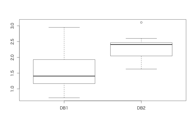
The result p < 0.05 allows us to conclude that DB1 is faster than DB2.*1
Chi-squared test
This is a method for comparing "ratio" between conditions, e.g. conversion rate (CVR). For example, imagine you modified possible conversion paths in your smartphone app and then you saw the count of CV as below:
| CV | non CV | |
|---|---|---|
| Before | 25 | 117 |
| After | 16 | 32 |
In the case of "tabulated" datasets like this example, we cannot compare the "ratio" with considering any kinds of variability computed from raw and unaggregated datasets like t-test. Instead, we can run chi-squared test (test of independency) that compares whether both datasets are generated from a unique and identical distribution.
> d<-matrix(c(25,117,16,32),ncol=2,byrow=T)
> chisq.test(d) # chisq.test() for chi-squared test

	Pearson's Chi-squared test with Yates' continuity correction

data:  d
X-squared = 4.3556, df = 1, p-value = 0.03689
We got p < 0.05 and can conclude that your modification significantly increases CV. FYI, when you have a series of results from multiple chi-squared test with the same intervention in distinct datasets, you can integrate them with Cochran-Mantel-Haenszel test. Of course, in case of t-test, you can also integrate with Rosenthal's method. Such meta-analysis techniques are very useful so please check them by yourself. :)
ANOVA (Analysis of Variance)
In principle, this method is an integrated version of t-test on more than 2 datasets and used when you want to compare means across more than 2 datasets with more than 1 intervention. This is a variant of multivariate analysis such as multiple regression (linear models). In particular ANOVA says whether there is a "main effect" and "interaction" of/between interventions (explanatory variables), and those are almost identical to coefficients in multiple regression. If you are interested in only whether there is any effect of interventions, ANOVA is the best; but if you are interested in both magnitude and direction of effects, you should use multiple regression.
Imagine you were selling 2 kinds of products at a department store in person: during 4 days, you were changing 2 kinds of promotion and now you want to know whether the type of promotion varies its revenue. Here we assume that variable 'pr' means which kind of promotion was used, 'category' means the category of product and 'cnt' means the revenue (dependent variable). You can compute an ANOVA model in R as below.
> d<-data.frame(cnt=c(210,435,130,720,320,470,250,380,290,505,180,320,310,390,410,510),pr=c(rep(c('F','Y'),8)),category=rep(c('a','a','b','b'),4))
> d.aov<-aov(cnt~.^2,d) # aov() function for ANOVA
> summary(d.aov)
            Df Sum Sq Mean Sq F value  Pr(>F)
pr           1 166056  166056  12.984 0.00362 **
category     1     56      56   0.004 0.94822
pr:category  1   5256    5256   0.411 0.53353
Residuals   12 153475   12790
---
Signif. codes:  0 ‘***’ 0.001 ‘**’ 0.01 ‘*’ 0.05 ‘.’ 0.1 ‘ ’ 1
We can conclude that the promotion has a 'main effect' which means the promotion significantly increase or decrease revenue. On the other hand, there is either no difference between the categories or no interaction between the category and the promotion.
Other hypothesis testing
We are also using other testing such as F-test, rank-sum test (Wilcoxon / Mann-Whitney test) and even we have to be aware of difference between parametric tests (requiring assumption of distribution of datasets and its shape) and nonparametric tests (requires no assumption), but all of them are a little advanced issues so I won't explain them here.
Multiple Regression (Linear Models)
I think this is one of the most basic methods in data science, but I feel it's still not so popular in practical business analytics although linear models are known as very easy methods in machine learning community and widely used for such machine learning systems even for business.
Below is an example of revenue of a beer brand in a certain district. Let's build a model for "Revenue" (of the beer per day) as a dependent variable with "CM" (a volume of TVCM per day), "Temp" (airtemperature) and "Firework" (categorical variable indicating whether there were any fireworks show in the district) as independent variables.
> d<-read.csv('https://raw.githubusercontent.com/ozt-ca/tjo.hatenablog.samples/master/r_samples/public_lib/DM_sampledata/ch4_3_2.txt',header=T,sep=' ')
> head(d)
   Revenue  CM Temp Firework
1 47.14347 141   31        2
2 36.92363 144   23        1
3 38.92102 155   32        0
4 40.46434 130   28        0
5 51.60783 161   37        0
6 32.87875 154   27        0
> d.lm<-lm(Revenue~.,d) # lm() function for linear models
> summary(d.lm)

Call:
lm(formula = Revenue ~ ., data = d)

Residuals:
   Min     1Q Median     3Q    Max
-6.028 -3.038 -0.009  2.097  8.141

Coefficients:
            Estimate Std. Error t value Pr(>|t|)
(Intercept) 17.23377   12.40527   1.389  0.17655
CM          -0.04284    0.07768  -0.551  0.58602
Temp         0.98716    0.17945   5.501    9e-06 ***
Firework     3.18159    0.95993   3.314  0.00271 **
---
Signif. codes:  0 ‘***’ 0.001 ‘**’ 0.01 ‘*’ 0.05 ‘.’ 0.1 ‘ ’ 1

Residual standard error: 3.981 on 26 degrees of freedom
Multiple R-squared:  0.6264,	Adjusted R-squared:  0.5833
F-statistic: 14.53 on 3 and 26 DF,  p-value: 9.342e-06

# Plotting
> matplot(cbind(d$Revenue,predict(d.lm,newdata=d[,-1])),type='l',lwd=c(2,3),lty=1,col=c(1,2))
> legend('topleft',legend=c('Data','Predicted'),lwd=c(2,3),lty=1,col=c(1,2),ncol=1)
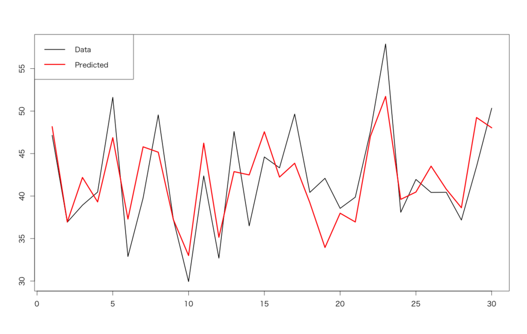
We can conclude that temperature and whether there were fireworks shows on each day are important. Of course if we can obtain any future values of the independent variables (indeed TVCM are planned in advance and temperature are officially forecasted), we can forecast future revenue with predict() method.
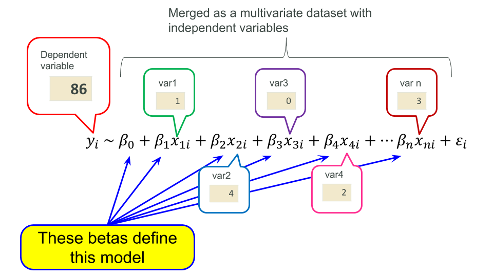
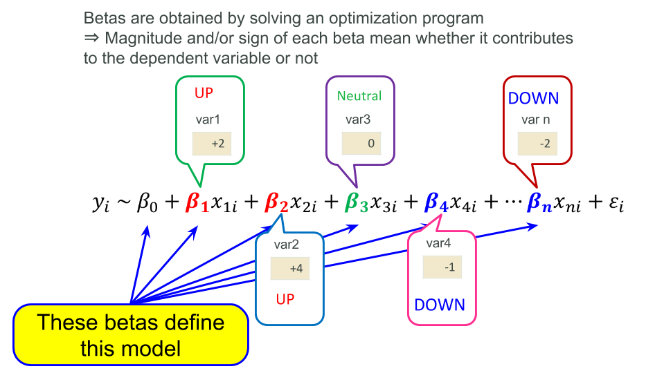
In short, linear modeling is a method representing a dependent variable with summation of products of independent variables and coefficients (parameters ββ) that are estimated with optimization programming. This idea is common across most of statistical modeling and even machine learning (in particular logistic regression and/or many online learning algorithms), so please keep them in mind.
(Notice: a lot of textbooks refer linear models as a 'basic' model of machine learning. In many implementations parameters are directly estimated by matrix calculation, but I recommend to implement an algorithm with the gradient descent in Python or other script languages in order to understand what it works)
General Linear Models (GLM: logistic regression, Poisson regression)
I think GLM is at the border between statistics and machine learning, and also one of the most interesting matter in statistical modeling. It is almost the same as linear models, but in GLM its dependent variable is NOT assumed to be normally distributed; we have to care about how it should be distributed, e.g. with Poisson distribution, Negative-binomial distribution, etc.
Logistic Regression
This is a binary classification and also a basic but important method in machine learning. Its dependent variable is distributed with binomial distribution. Below is an example from the chapter 6 of my textbook, in which "cv" is the dependent variable as the count of conversion of a certain e-commerce service and "d21-d26" are the independent variables as distinct promotion pages. We are supposed to clarify which promotion page contributes to CV.
> d<-read.csv('https://raw.githubusercontent.com/ozt-ca/tjo.hatenablog.samples/master/r_samples/public_lib/DM_sampledata/ch6_4_2.txt',header=T,sep=' ')
> d$cv<-as.factor(d$cv) # Casting cv to categorical
> d.glm<-glm(cv~.,d,family=binomial) # "family" argument handles what kind of distribution should be used
> summary(d.glm)

Call:
glm(formula = cv ~ ., family = binomial, data = d)

Deviance Residuals:
    Min       1Q   Median       3Q      Max
-2.3793  -0.3138  -0.2614   0.4173   2.4641

Coefficients:
            Estimate Std. Error z value Pr(>|z|)
(Intercept)  -1.0120     0.9950  -1.017   0.3091
d21           2.0566     0.8678   2.370   0.0178 *
d22          -1.7610     0.7464  -2.359   0.0183 *
d23          -0.2136     0.6131  -0.348   0.7276
d24           0.2994     0.8368   0.358   0.7205
d25          -0.3726     0.6064  -0.614   0.5390
d26           1.4258     0.6408   2.225   0.0261 *
---
Signif. codes:  0 ‘***’ 0.001 ‘**’ 0.01 ‘*’ 0.05 ‘.’ 0.1 ‘ ’ 1

(Dispersion parameter for binomial family taken to be 1)

    Null deviance: 173.279  on 124  degrees of freedom
Residual deviance:  77.167  on 118  degrees of freedom
AIC: 91.167

Number of Fisher Scoring iterations: 5
We can conclude that "d21" is the best and "d22" is the worst. Of course this model can forecast future dependent variable with predict() method and independent variables in the future.
Poisson Regression
In contrast to logistic regression, Poisson regression is rather statistical modeling than machine learning, used in the case that its dependent variable is distributed with Poisson distribution. You'll see a lot of definition and/or examples about Poisson distribution if you're Googling, but in principle it represents counts of some "rare" events. For example, a histogram as below means Poisson distribution.
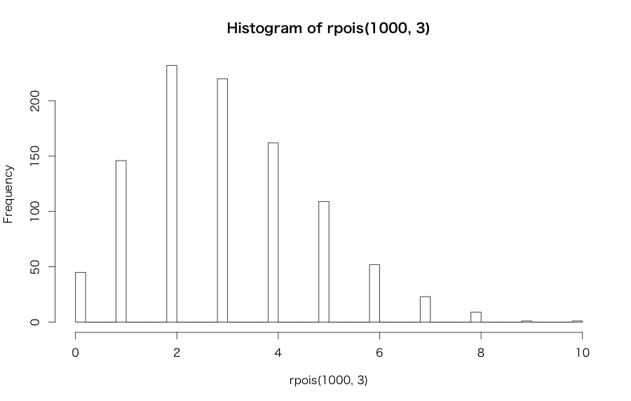
In actual business scenes, the number of conversions per day against the number of page views at a certain web site is the most famous example distributed as Poisson distribution*2.
By the way, very unfortunately I have no good example for Poisson regression... so here let's use the original example raised in R help :( According to the help, this dataset is from "An Introduction to Generalized Linear Models" by Dobson in 1990.
> ## Dobson (1990) Page 93: Randomized Controlled Trial :
> counts <- c(18,17,15,20,10,20,25,13,12)
> outcome <- gl(3,1,9)
> treatment <- gl(3,3)
> print(d.AD <- data.frame(treatment, outcome, counts))
  treatment outcome counts
1         1       1     18
2         1       2     17
3         1       3     15
4         2       1     20
5         2       2     10
6         2       3     20
7         3       1     25
8         3       2     13
9         3       3     12
> glm.D93 <- glm(counts ~ outcome + treatment, family = poisson) # "family" argument should be "poisson"
> summary(glm.D93)

Call:
glm(formula = counts ~ outcome + treatment, family = poisson)

Deviance Residuals:
       1         2         3         4         5         6         7         8         9
-0.67125   0.96272  -0.16965  -0.21999  -0.95552   1.04939   0.84715  -0.09167  -0.96656

Coefficients:
              Estimate Std. Error z value Pr(>|z|)
(Intercept)  3.045e+00  1.709e-01  17.815   <2e-16 ***
outcome2    -4.543e-01  2.022e-01  -2.247   0.0246 *
outcome3    -2.930e-01  1.927e-01  -1.520   0.1285
treatment2   1.338e-15  2.000e-01   0.000   1.0000
treatment3   1.421e-15  2.000e-01   0.000   1.0000
---
Signif. codes:  0 ‘***’ 0.001 ‘**’ 0.01 ‘*’ 0.05 ‘.’ 0.1 ‘ ’ 1

(Dispersion parameter for poisson family taken to be 1)

    Null deviance: 10.5814  on 8  degrees of freedom
Residual deviance:  5.1291  on 4  degrees of freedom
AIC: 56.761

Number of Fisher Scoring iterations: 4
# AIC gives how the model is generalized and a ratio of Residual deviance and degrees of freedom indicates how the model is overdispersed.
# If the ratio is too larger than 1, it's overdispersed

> hist(counts,breaks=50)
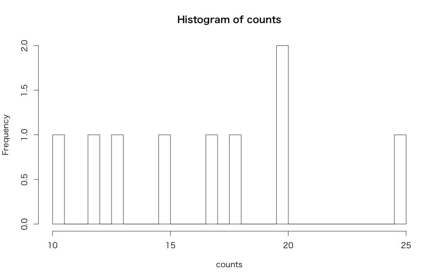
The result shows outcome2 is important. In general, Poisson regression may not work well when dependent variable includes too many zeros (overdispersion), so in such a case you have to use negative-binomial regression instead of Poisson regression. {VGAM} package provides glm.nb() function for negative-binomial regression.
Regularization / Penalization (L1 / L2 norm)
Just in my opinion, but regularization / penalization is rather machine learning matter than statistical one.
"Generalization" is a term representing to what extent a model fits not only training data but also test data. Regularization is one of the strong methods to generalize a model: in general, when you apply some generalization, parameters of a model will be estimated with a certain restriction in order to prevent them from overfitting.
In particular, "splitting test dataset from training dataset" (cross validation) is very much important in machine learning. If not, obtained models may fit not only training data themselves but also a lot of "noises" with them. Cross validation has some variation, e.g. holdout, leave-one-out, k-folds, etc.
Here I tried Lasso regression (L1-regularized logistic regression) onto a dataset names "Tennis", distributed by UC Irvine ML repository. Men's dataset is used for training and women's dataset is used for test as hold-out cross validation. Lasso regression is a method cutting unnecessary independent variables.
> dm<-read.csv('https://github.com/ozt-ca/tjo.hatenablog.samples/raw/master/r_samples/public_lib/jp/exp_uci_datasets/tennis/men.txt',header=T,sep='\t')
> dw<-read.csv('https://github.com/ozt-ca/tjo.hatenablog.samples/raw/master/r_samples/public_lib/jp/exp_uci_datasets/tennis/women.txt',header=T,sep='\t')
> dm<-dm[,-c(1,2,16,17,18,19,20,21,34,35,36,37,38,39)]
> dw<-dw[,-c(1,2,16,17,18,19,20,21,34,35,36,37,38,39)]

# L1 regularization
> library(glmnet)
> dm.cv.glmnet<-cv.glmnet(as.matrix(dm[,-1]),as.matrix(dm[,1]),family="binomial",alpha=1)
# alpha=1 for L1 regularization, alpha=0 for L2 regularization, and (0, 1) for elastic net
# cv.glmnet() function optimizes a parameter with cross validation

> plot(dm.cv.glmnet)
> coef(dm.cv.glmnet,s=dm.cv.glmnet$lambda.min) # "s" argument requires the optimized parameter
25 x 1 sparse Matrix of class "dgCMatrix"
                        1
(Intercept)  3.533402e-01
FSP.1        3.805604e-02
FSW.1        1.179697e-01
SSP.1       -3.275595e-05
SSW.1        1.475791e-01
ACE.1        .
DBF.1       -8.934231e-02
WNR.1        3.628403e-02
UFE.1       -7.839983e-03
BPC.1        3.758665e-01
BPW.1        2.064167e-01
NPA.1        .
NPW.1        .
FSP.2       -2.924528e-02
FSW.2       -1.568441e-01
SSP.2        .
SSW.2       -1.324209e-01
ACE.2        1.233763e-02
DBF.2        4.032510e-02
WNR.2       -2.071361e-02
UFE.2       -6.114823e-06
BPC.2       -3.648171e-01
BPW.2       -1.985184e-01
NPA.2        .
NPW.2        1.340329e-02
> table(dw$Result,round(predict(dm.cv.glmnet,as.matrix(dw[,-1]),s=dm.cv.glmnet$lambda.min,type='response'),0))

      0   1
  0 215  12
  1  18 207
> sum(diag(table(dw$Result,round(predict(dm.cv.glmnet,as.matrix(dw[,-1]),s=dm.cv.glmnet$lambda.min,type='response'),0))))/nrow(dw)
[1] 0.9336283 # Accuracy 93.4 %

# Comparison: case of usual logistic regression
> dm.glm<-glm(Result~.,dm,family=binomial)
> table(dw$Result,round(predict(dm.glm,newdata=dw[,-1],type

