机器学习作业(七)非监督学习——Matlab实现
题目下载【传送门】
第1题
简述:实现K-means聚类,并应用到图像压缩上。
第1步:实现kMeansInitCentroids函数,初始化聚类中心:
function centroids = kMeansInitCentroids(X, K)

% You should return this values correctly
centroids = zeros(K, size(X, 2));

randidx = randperm(size(X, 1));
centroids = X(randidx(1:K), :);

end
第2步:实现findClosestCentroids函数,进行样本点的分类:
function idx = findClosestCentroids(X, centroids)

% Set K
K = size(centroids, 1);

% You need to return the following variables correctly.
idx = zeros(size(X,1), 1);

for i = 1:size(X, 1),
    indexMin = 1;
    valueMin = norm(X(i,:) - centroids(1,:));
    for j = 2:K,
        valueTemp = norm(X(i,:) - centroids(j,:));
        if valueTemp < valueMin,
            valueMin = valueTemp;
            indexMin = j;
        end
    end
    idx(i, 1) = indexMin;
end

end
第3步:实现computeCentroids函数,计算聚类中心:
function centroids = computeCentroids(X, idx, K)

% Useful variables
[m n] = size(X);

% You need to return the following variables correctly.
centroids = zeros(K, n);


centSum = zeros(K, n);
centNum = zeros(K, 1);
for i = 1:m,
    centSum(idx(i, 1), :) = centSum(idx(i, 1), :) + X(i, :);
    centNum(idx(i, 1), 1) = centNum(idx(i, 1), 1) + 1;
end
for i = 1:K,
    centroids(i, :) = centSum(i, :) ./ centNum(i, 1);
end

end
第4步:实现runkMeans函数,完成k-Means聚类:
function [centroids, idx] = runkMeans(X, initial_centroids, ...
                                      max_iters, plot_progress)

% Set default value for plot progress
if ~exist('plot_progress', 'var') || isempty(plot_progress)
    plot_progress = false;
end

% Plot the data if we are plotting progress
if plot_progress
    figure;
    hold on;
end

% Initialize values
[m n] = size(X);
K = size(initial_centroids, 1);
centroids = initial_centroids;
previous_centroids = centroids;
idx = zeros(m, 1);

% Run K-Means
for i=1:max_iters

    % Output progress
    fprintf('K-Means iteration %d/%d...\n', i, max_iters);
    if exist('OCTAVE_VERSION')
        fflush(stdout);
    end

    % For each example in X, assign it to the closest centroid
    idx = findClosestCentroids(X, centroids);

    % Optionally, plot progress here
    if plot_progress
        plotProgresskMeans(X, centroids, previous_centroids, idx, K, i);
        previous_centroids = centroids;
        fprintf('Press enter to continue.\n');
        pause;
    end

    % Given the memberships, compute new centroids
    centroids = computeCentroids(X, idx, K);
end

% Hold off if we are plotting progress
if plot_progress
    hold off;
end

end
第5步:读取数据文件,完成二维数据的聚类:
% Load an example dataset
load('ex7data2.mat');

% Settings for running K-Means
K = 3;
max_iters = 10;
initial_centroids = [3 3; 6 2; 8 5];

% Run K-Means algorithm. The 'true' at the end tells our function to plot
% the progress of K-Means
[centroids, idx] = runkMeans(X, initial_centroids, max_iters, true);
fprintf('\nK-Means Done.\n\n');
运行结果:

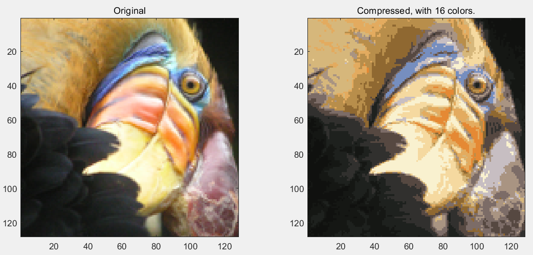
第6步:读取图片文件,完成图片颜色的聚类,转为16种颜色:
%  Load an image of a bird
A = double(imread('bird_small.png'));

% If imread does not work for you, you can try instead
%   load ('bird_small.mat');

A = A / 255; % Divide by 255 so that all values are in the range 0 - 1

% Size of the image
img_size = size(A);

% Reshape the image into an Nx3 matrix where N = number of pixels.
% Each row will contain the Red, Green and Blue pixel values
% This gives us our dataset matrix X that we will use K-Means on.
X = reshape(A, img_size(1) * img_size(2), 3);

% Run your K-Means algorithm on this data
% You should try different values of K and max_iters here
K = 16;
max_iters = 10;

% When using K-Means, it is important the initialize the centroids
% randomly.
% You should complete the code in kMeansInitCentroids.m before proceeding
initial_centroids = kMeansInitCentroids(X, K);

% Run K-Means
[centroids, idx] = runkMeans(X, initial_centroids, max_iters);

fprintf('Program paused. Press enter to continue.\n');
pause;

% Find closest cluster members
idx = findClosestCentroids(X, centroids);

% We can now recover the image from the indices (idx) by mapping each pixel
% (specified by its index in idx) to the centroid value
X_recovered = centroids(idx,:);

% Reshape the recovered image into proper dimensions
X_recovered = reshape(X_recovered, img_size(1), img_size(2), 3);

% Display the original image
subplot(1, 2, 1);
imagesc(A);
title('Original');

% Display compressed image side by side
subplot(1, 2, 2);
imagesc(X_recovered)
title(sprintf('Compressed, with %d colors.', K));
运行结果:
第2题
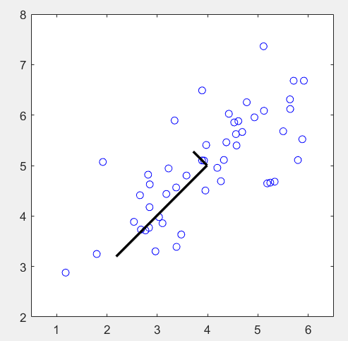
简述:使用PCA算法,完成维度约减,并应用到图像处理和数据显示上。
第1步:读取数据文件,并可视化:
%  The following command loads the dataset. You should now have the
%  variable X in your environment
load ('ex7data1.mat');

%  Visualize the example dataset
plot(X(:, 1), X(:, 2), 'bo');
axis([0.5 6.5 2 8]); axis square;
第2步:对数据进行归一化,计算协方差矩阵Sigma,并求其特征向量:
%  Before running PCA, it is important to first normalize X
[X_norm, mu, sigma] = featureNormalize(X);

%  Run PCA
[U, S] = pca(X_norm);

%  Compute mu, the mean of the each feature

%  Draw the eigenvectors centered at mean of data. These lines show the
%  directions of maximum variations in the dataset.
hold on;
drawLine(mu, mu + 1.5 * S(1,1) * U(:,1)', '-k', 'LineWidth', 2);
drawLine(mu, mu + 1.5 * S(2,2) * U(:,2)', '-k', 'LineWidth', 2);
hold off;
其中featureNormalize函数:
function [X_norm, mu, sigma] = featureNormalize(X)

mu = mean(X);
X_norm = bsxfun(@minus, X, mu);

sigma = std(X_norm);
X_norm = bsxfun(@rdivide, X_norm, sigma);

end
其中pca函数:
function [U, S] = pca(X)

% Useful values
[m, n] = size(X);

% You need to return the following variables correctly.
U = zeros(n);
S = zeros(n);

Sigma = 1 / m * (X' * X);
[U, S, V] = svd(Sigma);

end
运行结果:
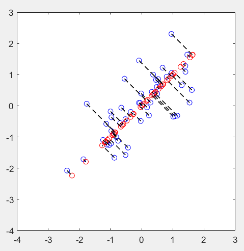
第3步:实现维度约减,并还原:
%  Plot the normalized dataset (returned from pca)
plot(X_norm(:, 1), X_norm(:, 2), 'bo');
axis([-4 3 -4 3]); axis square

%  Project the data onto K = 1 dimension
K = 1;
Z = projectData(X_norm, U, K);

X_rec  = recoverData(Z, U, K);

%  Draw lines connecting the projected points to the original points
hold on;
plot(X_rec(:, 1), X_rec(:, 2), 'ro');
for i = 1:size(X_norm, 1)
    drawLine(X_norm(i,:), X_rec(i,:), '--k', 'LineWidth', 1);
end
hold off
其中projectData函数:
function Z = projectData(X, U, K)

% You need to return the following variables correctly.
Z = zeros(size(X, 1), K);

Ureduce = U(:, 1:K);
Z = X * Ureduce;

end
其中recoverData函数:
function X_rec = recoverData(Z, U, K)

X_rec = zeros(size(Z, 1), size(U, 1));

Ureduce = U(:, 1:K);
X_rec = Z * Ureduce';

end
运行结果:
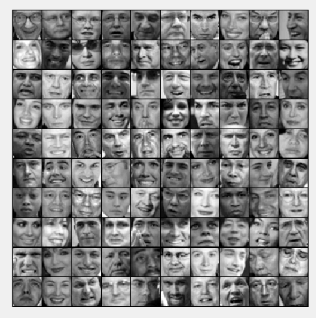
第4步:加载人脸数据,并可视化:
%  Load Face dataset
load ('ex7faces.mat')

%  Display the first 100 faces in the dataset
displayData(X(1:100, :));
运行结果:
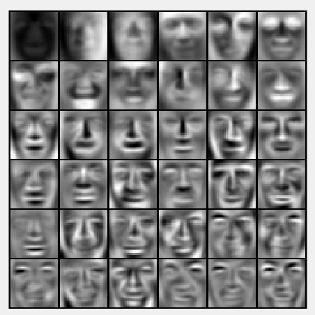
第5步:计算协方差矩阵的特征向量,并可视化:
%  Before running PCA, it is important to first normalize X by subtracting
%  the mean value from each feature
[X_norm, mu, sigma] = featureNormalize(X);

%  Run PCA
[U, S] = pca(X_norm);

%  Visualize the top 36 eigenvectors found
displayData(U(:, 1:36)');
运行结果:
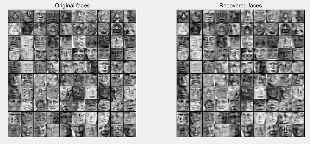
第6步:实现维度约减和复原:
K = 100;
Z = projectData(X_norm, U, K);
X_rec  = recoverData(Z, U, K);

% Display normalized data
subplot(1, 2, 1);
displayData(X_norm(1:100,:));
title('Original faces');
axis square;

% Display reconstructed data from only k eigenfaces
subplot(1, 2, 2);
displayData(X_rec(1:100,:));
title('Recovered faces');
axis square;
运行结果:
第7步:对图片的3维数据进行聚类,并随机挑选1000个点可视化:
% Reload the image from the previous exercise and run K-Means on it
% For this to work, you need to complete the K-Means assignment first
A = double(imread('bird_small.png'));

A = A / 255;
img_size = size(A);
X = reshape(A, img_size(1) * img_size(2), 3);
K = 16;
max_iters = 10;
initial_centroids = kMeansInitCentroids(X, K);
[centroids, idx] = runkMeans(X, initial_centroids, max_iters);

%  Sample 1000 random indexes (since working with all the data is
%  too expensive. If you have a fast computer, you may increase this.
sel = floor(rand(1000, 1) * size(X, 1)) + 1;

%  Setup Color Palette
palette = hsv(K);
colors = palette(idx(sel), :);

%  Visualize the data and centroid memberships in 3D
figure;
scatter3(X(sel, 1), X(sel, 2), X(sel, 3), 10, colors);
title('Pixel dataset plotted in 3D. Color shows centroid memberships');
运行结果:

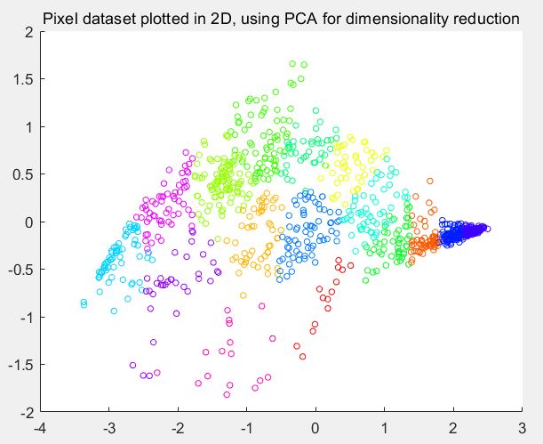
第8步:将数据降为2维:
% Subtract the mean to use PCA
[X_norm, mu, sigma] = featureNormalize(X);

% PCA and project the data to 2D
[U, S] = pca(X_norm);
Z = projectData(X_norm, U, 2);

% Plot in 2D
figure;
plotDataPoints(Z(sel, :), idx(sel), K);
title('Pixel dataset plotted in 2D, using PCA for dimensionality reduction');
运行结果:

 浙公网安备 33010602011771号