

1.keras实现-->使用预训练的卷积神经网络(VGG16)
VGG16内置于Keras,可以通过keras.applications模块中导入。
--------------------------------------------------------将VGG16 卷积实例化:-------------------------------------------------------------------------------------------------------------------------------------
1 from keras.applications import VGG16
2
3 conv_base = VGG16(weights = 'imagenet',#指定模型初始化的权重检查点
4                   include_top = False,
5                   input_shape = (150,150,30))
weights:指定模型初始化的权重检查点、
include_top: 指定模型最后是否包含密集连接分类器。默认情况下,这个密集连接分类器对应于ImageNet的100个类别。如果打算使用自己的密集连接分类器,可以不适用它,置为False。
input_shape: 是输入到网络中的图像张量的形状。这个参数完全是可选的,如果不传入这个参数,那么网络能够处理任意形状的输入。
--------------------------------------------------------查看VGG详细架构:conv_base.summary()----------------------------------------------------------------------------------------------------------
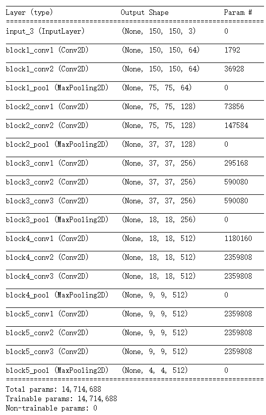
最后一特征图形状为(4,4,512),我们将在这个特征上添加一个密集连接分类器,有两种方式:
|
方法一:在你的数据集上运行卷积基,将输出保存为numpy数组,然后用这个数据做输入,输入到独立的密集连接分类器中。这种方法速度快,计算代价低,因为对于每个输入图像只需运行一次卷积基,而卷积基是日前流程中计算代价最高的。但这种方法不允许使用数据增强。 |
方法二:在顶部添加Dense层来扩展已有模型,并在输入数据上端到端地运行整个模型。这样你可以使用数据增强,因为每个输入图像进入模型时都会经过卷积基。但这种方法的计算代价比第一种要高很多。 |
|
#方法一:不使用数据增强的快速特征提取
import os
import numpy as np
from keras.preprocessing.image import ImageDataGenerator

base_dir = 'cats_dogs_images'

train_dir = os.path.join(base_dir,'train')
validation_dir = os.path.join(base_dir,'validation')
test_dir = os.path.join(base_dir,'test')

datagen = ImageDataGenerator(rescale = 1./255)#将所有图像乘以1/255缩放
batch_size = 20

def extract_features(directory,sample_count):
    features = np.zeros(shape=(sample_count,4,4,512))
    labels = np.zeros(shape=(sample_count))
# 通过.flow或.flow_from_directory(directory)方法实例化一个针对图像batch的生成器,这些生成器
# 可以被用作keras模型相关方法的输入,如fit_generator,evaluate_generator和predict_generator
    generator = datagen.flow_from_directory(
        directory,
        target_size = (150,150),
        batch_size = batch_size,
        class_mode = 'binary')
    i = 0
    for inputs_batch,labels_batch in generator:
        features_batch = conv_base.predict(inputs_batch)
        features[i * batch_size:(i+1) * batch_size] = features_batch
        labels[i * batch_size:(i+1)*batch_size] = labels_batch
        i += 1
        if i * batch_size >= sample_count:
            break
    return features,labels


train_features,train_labels = extract_features(train_dir,2000)
validation_features,validation_labels = extract_features(validataion_dir,1000)
test_features,test_labels = extract_features(test_dir,1000)

#要将特征(samples,4,4,512)输入密集连接分类器中,首先必须将其形状展平为(samples,8192)

train_features = np.reshape(train_features,(2000,4*4*512))
validation_features = np.reshape(validation_features,(2000,4*4*512))
test_features = np.reshape(test_features,(2000,4*4*512))

#定义并训练密集连接分类器
from keras import models
from keras import layers
from keras import optimizers

model = models.Sequential()
model.add(layers.Dense(256,activation='relu',input_dim=4*4*512))
model.add(layers.Dropout(0.5))
model.add(layers.Dense(1,activation='sigmoid'))

model.compile(optimizer=optimizers.RMSprop(lr=2e-5),
              loss='binary_crossentropy',
              metrics = ['acc'])

history = model.fit(train_features,train_labels,
                    epochs=30,batch_size=20,
                    validation_data = (validation_features,validation_labels) )
|
#在卷积基上添加一个密集连接分类器

from keras import models
from keras import layers

model = models.Sequential()
model.add(conv_base)
model.add(layers.Flatten())
model.add(layers.Dense(256,activation='relu'))
model.add(layers.Dense(1,activation='sigmoid'))

model.summary()
在编译和训练模型之前,一定要“冻结”卷积基。 冻结☞ 指一个或多个层在训练过程中保持其权重不变 如果不这么做,那么卷积基之前学到的表示将会在训练过程中被修改。因为其上添加的Dense层是随机初始化的,所以非常大的权重更新将会在网络中传播,对之前学到的表示造成很大破坏。 在keras中,冻结网络的方法是将其trainable属性设置为False eg. conv_base.trainable = False
#使用冻结的卷积基端到端地训练模型
|
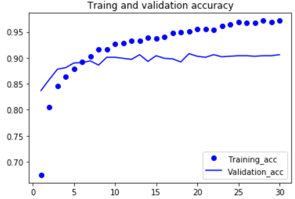
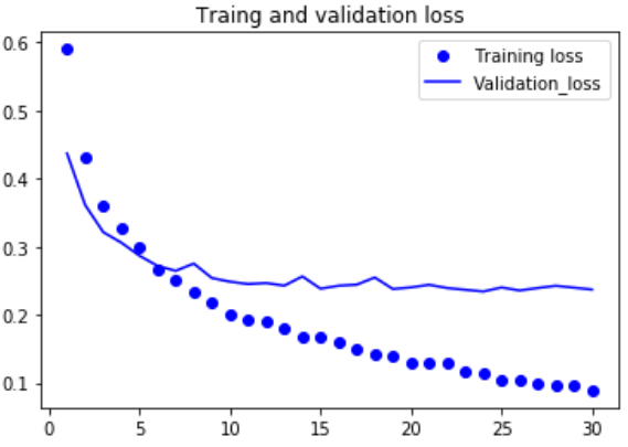
#绘制损失曲线和精度曲线
import matplotlib.pyplot as plt

acc = history.history['acc']
val_acc = history.history['val_acc']
loss = history.history['loss']
val_loss = history.history['val_loss']

epochs = range(1,len(acc)+1)

plt.plot(epochs,acc,'bo',label='Training_acc')
plt.plot(epochs,val_acc,'b',label='Validation_acc')
plt.title('Traing and validation accuracy')
plt.legend()

plt.figure()

plt.plot(epochs,loss,'bo',label='Training loss')
plt.plot(epochs,val_loss,'b',label='Validation_loss')
plt.title('Traing and validation loss')
plt.legend()

plt.show()
|
|
|
|
电脑带不起来,慢死,这边就不截图了。 验证精度约为96% |

--------------------------------------------------------微调模型--------------------------------------------------------------------------------------------------------------------------------------------------------------
另外一种广泛使用的模型复用方法是模型微调,与特征提取互为补充。
对于用于特征提取的冻结的模型基,微调是指将其顶部的几层“解冻”,并将这解冻的几层和新增加的部分联合训练。之所以叫作微调,是因为他只是略微调整了所复用模型中更加抽象的表示,
以便让这些表示与手头的问题更加相关。
冻结VGG16的卷积基是为了能够在上面训练一个随机初始化的分类器。同理,只有上面的分类器训练好了,才能微调卷积基的顶部几层。如果分类器没有训练好,那么训练期间通过网络传播的
误差信号会特别大,微调的几层之前学到的表示都会被破坏。因此,微调网络的步骤如下:
(1)在已经训练好的基网络上添加自定义网络
(2)冻结基网络
(3)训练所添加的部分
(4)解冻基网络的一些层
(5)联合训练解冻的这些层和添加的部分
# 冻结直到某一层的所有层 #仅微调卷积基的最后的两三层 conv_base.trainable = True set_trainable = False for layer in conv_base.layers[:-1]: if layer.name == 'block5_conv1': set_trainable = True if set_trainable: print(layer) set_trainable = True else: set_trainable = False |
|
#微调模型 model.compile(loss='binary_crossentropy', optimizer = optimizers.RMSprop(lr=1e-5), metrics = ['acc']) history = model.fit_generator( train_generator, steps_per_epoch=10, epochs = 5, validation_data = validation_generator, validation_steps = 50 ) |
|
test_generator = test_datagen.flow_from_directory( test_dir, target_size = (150,150), batch_size = 20, class_mode = 'binary' ) test_loss,test_acc = model.evaluate_generator(test_generator,steps=50) |
得到了97%的测试精度
|
#使曲线变得平滑
def smooth_curve(points,factor = 0.2):
    smoothed_points = []
    for point in points:
        if smoothed_points:
            previous = smoothed_points[-1]
            smoothed_points.append(previous*factor+point*(1-factor))
        else:
            smoothed_points.append(point)
    return smoothed_points
|
为什么不微调更多层?为什么不微调整个卷积基?当然可以这么做,但需要先考虑以下几点:
(1)卷积基中更靠底部的层编码的是更加通用的可复用特征,而更靠顶部的层编码的是更专业化的特征。微调这些更专业化的特征更加有用,因为它们需要在你的新问题上改变用途。
微调更靠底部的层,得到的汇报会更少
(2)训练的参数越多,过拟合的风险越大。卷积基有1500万个参数,所以在你的小型数据集上训练这么多参数是有风险的。
--------------------------------------------------------卷积神经网络的可视化------------------------------------------------------------------------------------------------------------------------------------------------------------------------
三种最容易理解也最有用的方法:
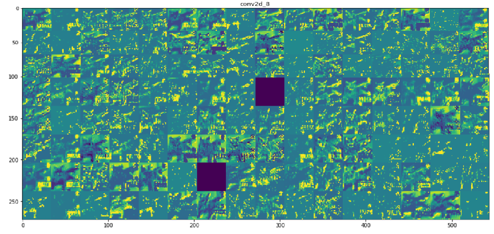
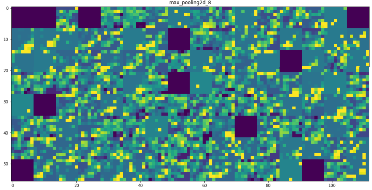
(1)可视化卷积神经网络的中间输出(中间激活):有助于理解卷积神经网络连续的层如何对输入进行变换,也有助于初步了解神经网络每个过滤器的含义
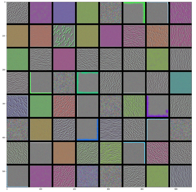
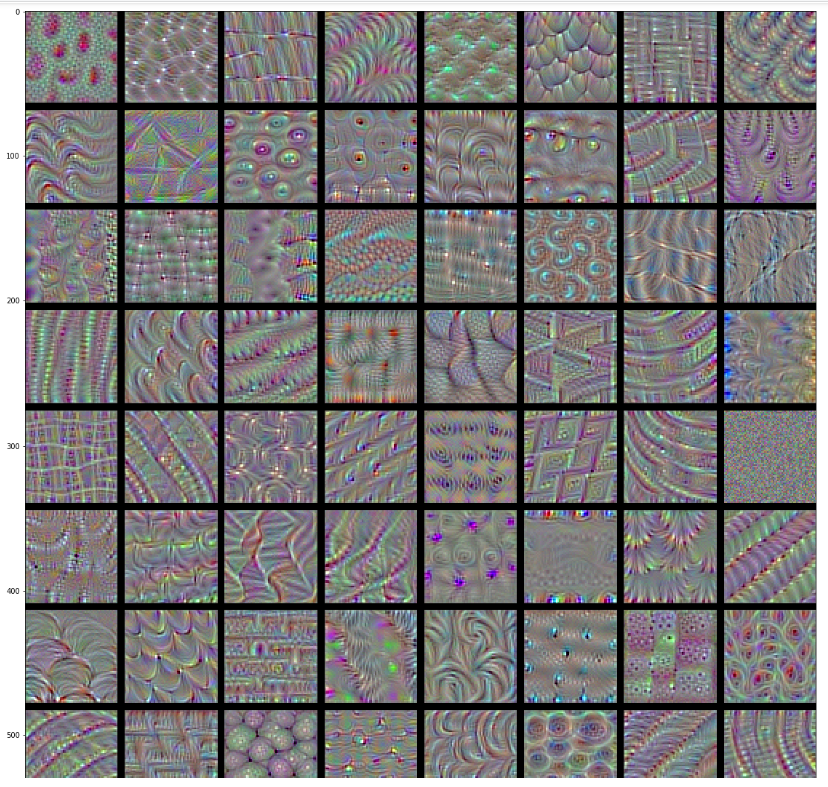
(2)可视化卷积神经网络的过滤器:有助于精确理解卷积神经网络中每个过滤器容易接受的视觉模式或视觉概念
(3)可视化图像中类激活的热力图:有助于理解图像的哪个部分被识别为属于哪个类别,从而可以定位图像中的物体
| 可视化卷积神经网络的中间输出(中间激活) | 可视化卷积神经网络的过滤器 |
|
from keras.models import load_model model = load_model('cats_and_dogs_small_2.h5') model.summary() |
#为过滤器的可视化定义损失张量 from keras.applications import VGG16 from keras import backend as K model = VGG16(weights = 'imagenet',include_top = False) def generate_pattern(layer_name,filter_index,size=150): layer_output = model.get_layer(layer_name).output loss = K.mean(layer_output[:,:,:,filter_index]) #获取损失相对于输入的梯度 grads = K.gradients(loss,model.input)[0] #梯度标准化 grads /= (K.sqrt(K.mean(K.square(grads))) + 1e-5)#1e-5防止不小心除以0 #给定numpy输入值,得到numpy输出值 iterate = K.function([model.input],[loss,grads]) #通过随机梯度下降让损失最大化 input_img_data = np.random.random((1,size,size,3))*20+128. step = 1. for i in range(40): loss_value,grads_value = iterate([input_img_data]) input_img_data += grads_value * step img = input_img_data[0] return deprocess_image(img) |
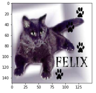
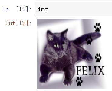
#预处理单张图像
img_path = 'cats_and_dogs_small/test/cats/cat.1501.jpg'

from keras.preprocessing import image
import numpy as np

img = image.load_img(img_path,target_size=(150,150))
img_tensor = image.img_to_array(img)
# img_tensor = np.expand_dims(img_tensor,axis=0)
img_tensor = img_tensor.reshape((1,)+img_tensor.shape)
img_tensor /= 255.

print(img_tensor.shape)
|
#将张量转化为有效图像的实用函数 def deprocess_image(x): x -= x.mean() x /= (x.std() + 1e-5) x *= 0.1 x += 0.5 x = np.clip(x,0,1) x *= 255 x = np.clip(x,0,255).astype('uint8') return x |
|
#显示测试图像 |
plt.imshow(generate_pattern('block3_conv1',0)) |
|

|
#用一个输入张量和一个输出张量列表将模型实例化
from keras import models

layer_outputs = [layer.output for layer in model.layers[:8]]
activation_model = models.Model(inputs=model.input,outputs=layer_outputs)#创建一个模型,给定模型输入,可以返回这些输出
#这个模型有一个输入和8个输出,即每层激活对于一个输出
|
#生成某一层中所有过滤器响应模式组成的网络
def create_vision(layer_name):
    size = 64
    margin = 5

    results = np.zeros((8 * size + 7 * margin , 8 * size + 7*margin ,3))
    for i in range(8):
        for j in range(8):
            filter_img = generate_pattern(layer_name, i + (j * 8), size = size)
            horizontal_start = i * size + i * margin
            horizontal_end = horizontal_start + size
            vertical_start = j*size + j * margin
            vertical_end = vertical_start + size
            results[horizontal_start:horizontal_end, vertical_start:vertical_end, :] = filter_img
    plt.figure(figsize=(20, 20))
    plt.imshow(results.astype('uint8'))
#不知为何deprocess_image无效,使得results矩阵并不是uint8格式,故需要转换否则不显示
|
#以预测模式运行模型 activations = activation_model.predict(img_tensor) #返回8个numpy数组组成的列表,每个层激活对应一个numpy数组 first_layer_activation = activations[3] #first_layer_activation.shape--> 32个通道 (1, 148, 148, 32) import matplotlib.pyplot as plt plt.matshow(first_layer_activation[0,:,:,15],cmap='viridis') |
layer_name = 'block1_conv1'
|

|
layer_name = 'block4_conv1'
|
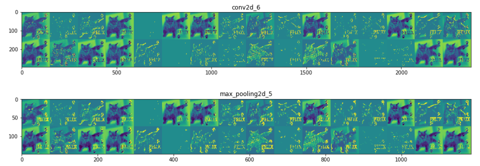
#将每个中间激活的所有通道可视化 layer_names = [] for layer in model.layers[:8]: layer_names.append(layer.name)#层的名字 images_per_row = 16 for layer_name,layer_activation in zip(layer_names,activations): n_features = layer_activation.shape[-1] #[32, 32, 64, 64, 128, 128, 128, 128] 特征个数 size = layer_activation.shape[1] #特征图的形状为(1,size,size,n_features) n_cols = n_features // images_per_row display_grid = np.zeros((size*n_cols,images_per_row*size)) for col in range(n_cols): for row in range(images_per_row): channel_image = layer_activation[0,:,:,col*images_per_row + row] channel_image -= channel_image.mean() channel_image /= channel_image.std() channel_image *= 64 channel_image += 128 channel_image = np.clip(channel_image,0,255).astype('uint8') display_grid[col*size:(col+1)*size,row*size:(row+1)*size]=channel_image scale = 1./size plt.figure(figsize=(scale*display_grid.shape[1], scale*display_grid.shape[0])) plt.title(layer_name) plt.grid(False) plt.imshow(display_grid,aspect='auto',cmap='viridis') |
|
|

可视化图像中类激活的热力图
|
|
|
from keras.applications import VGG16 model = VGG16(weights = 'imagenet',include_top = True) |
|
#为VGG16模型预处理一张输入图像 from keras.preprocessing import image from keras.applications.vgg16 import preprocess_input,decode_predictions import numpy as np img_path = 'E:/软件/nxf_software/pythonht/nxf_practice/keras/大象.jpg' img = image.load_img(img_path,target_size=(224,224))#读取图像并调整大小 x = image.img_to_array(img) # ==> array(150,150,3) plt.figure() implot = plt.imshow(image.array_to_img(x)) plt.show() |
|
x = x.reshape((1,)+x.shape) # ==> array(1,150,150,3)
x = preprocess_input(x)#对批量进行预处理(按通道进行颜色标准化)
preds = model.predict(x) decode_predictions(preds,top=3)[0]
|
|
 1 #为了展示图像中哪些部分最像非洲象,我们使用Grad-CAM算法
 2
 3 african_elephant_output = model.output[:386] #预测向量中的'非洲象'元素
 4
 5 last_conv_layer = model.get_layer('block5_conv3')#VGG16的最后一个卷积层
 6
 7 grads = K.gradients(african_elephant_output,last_conv_layer)[0]
 8
 9 iterate = K.function([model.input],[pooled_grads,last_conv_layer.output[0]])
10
11 pooled_grads_value,conv_layer_output_value = iterate([x])
12
13 for i in range(512):
14     conv_layer_output_value[:,:,i] *= pooled_grads_value[i]
15
16 headmap = np.mean(conv_layer_output_value,axis = -1)
|
|
|
heatmap = np.maximum(heatmap,0) headmap /= np.max(heatmap) plt.matshow(heatmap) |
|
 1 #将热力图与原始图像叠加
 2 import cv2
 3
 4 img = cv2.imread(img_path) #用cv2加载原始图像
 5
 6 heatmap = cv2.resize(heatmap,(img.shape[1],img.shape[0]))#将热力图的大小调整为与原始图像相同
 7
 8 heatmap = np.uint8(255 * heatmap)#将热力图转换为RGB格式
 9
10 heatmap = cv2.applyColorMap(heatmap,cv2.COLORMAP_JET)#将热力图应用于原始图像
11
12 superimposed_img = heatmap * 0.4 + img #0.4是热力图强度因子
13
14 cv2.imwrite('E:/软件/nxf_software/pythonht/nxf_practice/keras/大象1.jpg',superimposed_img) #将图像保存到硬盘
|
|
这种可视化方法回答了两个重要问题
|
|

 浙公网安备 33010602011771号