数据流环境下增量学习解决方案--sklearn-out_of_core_approach
sklearn关于out of core approach官方文档
数据流下的分类任务
提出问题
数据流环境下,概念漂移是普遍的现象,学习方法应该具有增量式的自适应学习新数据的能力。以适应不断变化的,不确定的动态环境。
具体而言,增量式学习(incremental learning)方式是指在训练样本不能全部获取的场景下,先在已有样本建立分类模型,再根据不断到来的新实例来修正或更新已有分类模型,从而使分类模型能不断适应最新的数据。在数据流研究领域,Gmma等人把这种适应概念漂移的能力的学习方法称为自适应学习技术。
类比上面提到的数据流场景,我们在现实模型的训练过程中会遇到下面两种情况:
- 可能短时间内拿不到所有的数据;
- 数据量太多的时候。训练模型的时候会出现Memory Error的错误;
在这两种情况下,我们不能舍弃数据的价值,因为我们需要数据来不断的给我们构建的模型提供信息以达到更好的效果。我们需要这种incremental learning的思想。这是数据流挖掘任务要处理的场景之一。
问题初步的解决办法:
使用sklearn中自称为out-of-core 的方法去解决上面的问题
首先需要一个支持partial_fit方法的分类器
然后将数据进行分批次的提供给模型,模型使用partial_fit方法进行训练
在sklearn中一些模型是提供了partial_fit方法的。这些模型都能够作为online classifier使用。
hasattr(clf, "partial_fit") #使用模型之前判断是不是带有partial_fit方法
Experiment (实验代码是在jupyter notebook上进行)
1.准备数据集
使用Reuters-21578做这次实验,数据集在UCI ML respoitory采集。下面代码在第一次运行的时候将自动的对该数据集下载并解压。
from glob import glob
import itertools
import os.path
import re
import tarfile
import time
import sys

from html.parser import HTMLParser
from urllib.request import urlretrieve
from sklearn.datasets import get_data_home

def _not_in_sphinx():
    # Hack to detect whether we are running by the sphinx builder
    return '__file__' in globals()

class ReutersParser(HTMLParser):
    """Utility class to parse a SGML file and yield documents one at a time.

    下载来的数据集是很多的sgm文件,每一个sgml文件中包含很多”文章“,一个文章也就是我们数据流中的一个样本点,
    我们需要的是title+body(文章标题+内容)和 topics(文章所属类别)。

    解析sgml文件,实例化类之后,调用对象的parse方法得到的一个generator,每次yield一个样本点出来
    """

    def __init__(self, encoding='latin-1'):
        HTMLParser.__init__(self)
        self._reset()
        self.encoding = encoding

    def handle_starttag(self, tag, attrs):
        method = 'start_' + tag
        getattr(self, method, lambda x: None)(attrs)

    def handle_endtag(self, tag):
        method = 'end_' + tag
        getattr(self, method, lambda: None)()

    def _reset(self):
        self.in_title = 0
        self.in_body = 0
        self.in_topics = 0
        self.in_topic_d = 0
        self.title = ""
        self.body = ""
        self.topics = []
        self.topic_d = ""

    def parse(self, fd):
        self.docs = []
        self.docs = []
        # 对文件内容做缓冲处理
        # 填充一些文本到解析器中。如果包含完整的元素,则被处理;如果数据不完整,将被缓冲直到更多的数据被填充
        for chunk in fd:
            #缓冲--执行
            self.feed(chunk.decode(self.encoding))
            #执行完之后会保存到对象的docs属性中,构造一个生成器,使用的时候每次yield一个doc
            for doc in self.docs:
                yield doc
            self.docs = []
        self.close()

    def handle_data(self, data):
        if self.in_body:
            self.body += data
        elif self.in_title:
            self.title += data
        elif self.in_topic_d:
            self.topic_d += data

    def start_reuters(self, attributes):
        pass

    def end_reuters(self):
        self.body = re.sub(r'\s+', r' ', self.body)
        self.docs.append({'title': self.title,
                          'body': self.body,
                          'topics': self.topics})
        self._reset()

    def start_title(self, attributes):
        self.in_title = 1

    def end_title(self):
        self.in_title = 0

    def start_body(self, attributes):
        self.in_body = 1

    def end_body(self):
        self.in_body = 0

    def start_topics(self, attributes):
        self.in_topics = 1

    def end_topics(self):
        self.in_topics = 0

    def start_d(self, attributes):
        self.in_topic_d = 1

    def end_d(self):
        self.in_topic_d = 0
        self.topics.append(self.topic_d)
        self.topic_d = ""


def stream_reuters_documents(data_path=None):
    """Iterate over documents of the Reuters dataset.

    The Reuters archive will automatically be downloaded and uncompressed if
    the `data_path` directory does not exist.

    Documents are represented as dictionaries with 'body' (str),
    'title' (str), 'topics' (list(str)) keys.

    """

    DOWNLOAD_URL = ('http://archive.ics.uci.edu/ml/machine-learning-databases/'
                    'reuters21578-mld/reuters21578.tar.gz')
    ARCHIVE_FILENAME = 'reuters21578.tar.gz'

    if data_path is None:
        data_path = os.path.join(get_data_home(), "reuters")
    if not os.path.exists(data_path):
        """Download the dataset."""
        print("downloading dataset (once and for all) into %s" %
              data_path)
        os.mkdir(data_path)
				# 利用 urlretrieve()方法直接将远程数据下载到本地
        def progress(blocknum, bs, size):
            total_sz_mb = '%.2f MB' % (size / 1e6)
            current_sz_mb = '%.2f MB' % ((blocknum * bs) / 1e6)
            if _not_in_sphinx():
                sys.stdout.write(
                    '\rdownloaded %s / %s' % (current_sz_mb, total_sz_mb))

        archive_path = os.path.join(data_path, ARCHIVE_FILENAME)
        urlretrieve(DOWNLOAD_URL, filename=archive_path,
                    reporthook=progress)
        if _not_in_sphinx():
            sys.stdout.write('\r')
        print("untarring Reuters dataset...")
        tarfile.open(archive_path, 'r:gz').extractall(data_path)
        print("done.")

    parser = ReutersParser()
    for filename in glob(os.path.join(data_path, "*.sgm")):
        for doc in parser.parse(open(filename, 'rb')):
            yield doc
-
为了方便理解上面的代码,我从下载下来的sgm文件里面的截取两段出来,这一个
内的内容就相当于数据流中的一个instance,根据这个结构去构建自己解析器,用python自带的HTMLParser就能解析这种简单的。 一个HTMLParser 类的实例用来接受 HTML 数据,并在标记开始、标记结束、文本、注释和其他 元素标记出现的时候调用对应的方法。要实现具体的行为,请使用HTMLParser 的子类并重载其方法。更加具体的内容查阅Python文档中有关html.parser.HTMLParser的说明,这里只说明类中最重要的两个方法。
HTMLParser.feed(data)
填充一些文本到解析器中。如果包含完整的元素,则被处理;如果数据不完整,将被缓冲直到更多
的数据被填充,或者close() 被调用。data 必须为str 类型。HTMLParser.close()
如同后面跟着一个文件结束标记一样,强制处理所有缓冲数据。这个方法能被派生类重新定义,用
于在输入的末尾定义附加处理,但是重定义的版本应当始终调用基类HTMLParser 的close() 方
法。
</REUTERS>
<REUTERS TOPICS="YES" LEWISSPLIT="TRAIN" CGISPLIT="TRAINING-SET" OLDID="18149" NEWID="1731">
<DATE> 4-MAR-1987 15:06:37.82</DATE>
<TOPICS><D>grain</D></TOPICS>
<PLACES><D>usa</D><D>ussr</D></PLACES>
<PEOPLE></PEOPLE>
<ORGS></ORGS>
<EXCHANGES></EXCHANGES>
<COMPANIES></COMPANIES>
<UNKNOWN>
C G
f0508reute
u f BC-/RENEWAL-OF-U.S./USSR 03-04 0110</UNKNOWN>
<TEXT>
<TITLE>RENEWAL OF U.S./USSR GRAIN PACT SAID UNCERTAIN</TITLE>
<DATELINE> WASHINGTON, March 4 - </DATELINE><BODY>Prospects for renewal of the
five-year U.S./USSR grains agreement are uncertain at this
point, a Soviet trade official told Reuters.
The current trade imbalance between the United States and
the Soviet Union, high U.S. commodity prices, and increased
world grain production make a renewal of the supply agreement
next year less certain, Albert Melnikov, deputy trade
representative of the Soviet Union, said in an interview.
The current agreement expires on Sept 30, 1988.
Melnikov said that world grain markets are different than
when the first agreement was signed in 1975.
Statements from both U.S. and Soviet officials have
indicate that a long term grains agreement might not be as
attractive for both sides as it once was.
"We have had one agreement. We have had a second agreement,
but with the second agreement we've had difficulties with
prices," Melnikov said.
"I cannot give you any forecasts in response to the future
about the agreement.... I do not want to speculate on what will
happen after Sept 30, 1988," he said.
Melnikov noted that he has seen no indications from Soviet
government officials that they would be pushing for a renewal
of the agreement.
"The situation is different in comparison to three, five or
ten years ago ... We can produce more," he said.
Reuter
</BODY></TEXT>
</REUTERS>
<REUTERS TOPICS="YES" LEWISSPLIT="TRAIN" CGISPLIT="TRAINING-SET" OLDID="18150" NEWID="1732">
<DATE> 4-MAR-1987 15:07:16.19</DATE>
<TOPICS><D>earn</D></TOPICS>
<PLACES><D>usa</D></PLACES>
<PEOPLE></PEOPLE>
<ORGS></ORGS>
<EXCHANGES></EXCHANGES>
<COMPANIES></COMPANIES>
<UNKNOWN>
F
f0511reute
d f BC-DANAHER-<DHR>-EXPECTS 03-04 0096</UNKNOWN>
<TEXT>
<TITLE>DANAHER <DHR> EXPECTS EARNINGS INCREASE IN 1987</TITLE>
<DATELINE> WASHINGTON, March 4 - </DATELINE><BODY>Danaher Corp said it expects higher
earnings in 1987 versus 1986.
"We expect significant increases in earnings and revenues
in 1987," Steven Rales, Danaher chairman and chief executive
officer, said.
Earlier, the company reported 1986 net earnings of 15.4 mln
dlrs, or 1.51 dlrs a share, versus 13.5 mln dlrs, or 1.32 dlrs
a share, in 1985.
It also reported fourth quarter net of 7.3 mln dlrs, or 71
cts a share, up from 4.4 mln dlrs, or 43 cts a share, in the
previous year's fourth quarter.
Reuter
</BODY></TEXT>
</REUTERS>
-
urllib.request模块提供的urlretrieve()函数。urlretrieve()方法直接将远程数据下载到本地。
该方法返回一个包含两个元素的(filename, headers) 的元组,filename 表示保存到本地的路 径,header表示服务器的响应头
urlretrieve(url, filename=None, reporthook=None, data=None)
url:下载链接地址
filename:指定了保存本地路径,如果参数未指定,urllib会生成一个临时文件保存数据。
reporthook:是一个回调函数,当连接上服务器、以及相应的数据块传输完毕时会触发该回调,我们可以. 利用这个回调函数来显示当前的下载进度。
data:指post到服务器的数据
直接调用stream_reuters_documents()方法,将会将数据下载到本地,我直接在jupyter notebook上运行:
data_stream = stream_reuters_documents()
downloading dataset (once and for all) into /Users/dengjiguang/scikit_learn_data/reuters
untarring Reuters dataset...
done.
这样我们就准备好了我们的数据流了!接下来才是重头戏
2.数据处理及测试
因为我们的解决办法是要对数据进行了截取,分了很多”数据批次“,可能会在后面的数据批次中出现新的特征,比如在文本分类中,新的特征(新words)很大可能会出现在不同的数据批次中,所以为了保证模型训练数据的特征空间是一致的,这里使用了HashingVectorizer将每一个样本都映射到同样的特征空间中。
# 创建一个vectorizer,将数据映射到一个特征空间中,将数据特征的个数限制到一个合理的最大值
# n_features这里设置为2 ** 18

from sklearn.feature_extraction.text import HashingVectorizer

vectorizer = HashingVectorizer(decode_error='ignore', n_features=2 ** 18,
                               alternate_sign=False)

# Iterator over parsed Reuters SGML files.
data_stream = stream_reuters_documents()

# 我们这里实验是做二分类,即文章topic是"acq"类或者是其他所有类。"acq"作为positive class
# 选择 "acq"是因为它在Reuters文件中分布均匀。
# 对于自己要做的数据集,选择自己合适的测试数据集。
all_classes = np.array([0, 1])
positive_class = 'acq'

# 下面是sklearn中支持partial_fit方法的一些分类器,我们分别使用这些分类器做效果对比
from sklearn.linear_model import SGDClassifier
from sklearn.linear_model import PassiveAggressiveClassifier
from sklearn.linear_model import Perceptron
from sklearn.naive_bayes import MultinomialNB

partial_fit_classifiers = {
    'SGD': SGDClassifier(max_iter=5),
    'Perceptron': Perceptron(),
    'NB Multinomial': MultinomialNB(alpha=0.01),
    'Passive-Aggressive': PassiveAggressiveClassifier(),
}


def get_minibatch(doc_iter, size, pos_class=positive_class):
    """Extract a minibatch of examples, return a tuple X_text, y.

    Note: size is before excluding invalid docs with no topics assigned.
    文件中有些文章是没有标记topics的,这些无效数据不使用。
    所以这里size虽然是制定的批次中样本点的大小,但是因为要去除掉无效数据,批次的大小<=size

    函数直接返回的一个批次的样本点数据

    """
    data = [('{title}\n\n{body}'.format(**doc), pos_class in doc['topics'])
            for doc in itertools.islice(doc_iter, size)
            if doc['topics']]
    if not len(data):
        return np.asarray([], dtype=int), np.asarray([], dtype=int)
    X_text, y = zip(*data)
    return X_text, np.asarray(y, dtype=int)


def iter_minibatches(doc_iter, minibatch_size):
    """Generator of minibatches.
    每次yield一个批次的数据
    """
    X_text, y = get_minibatch(doc_iter, minibatch_size)
    while len(X_text):
        yield X_text, y
        X_text, y = get_minibatch(doc_iter, minibatch_size)
- zip函数在对数据进行处理的时候很常用,这里只用两个例子去说明其作用
>>> x = [1, 2, 3]
>>> y = [4, 5, 6]
>>> zipped = zip(x, y)
>>> list(zipped)
[(1, 4), (2, 5), (3, 6)]
我们首先选取一些数据作为测试数据
我们预计将其作为接下来模型训练过程中的验证集,在使用每一批次数据训练之后,对学习到的模型进行测试。我们想要得到是分类器的分类精度在批次训练过程中的演变。
# test data statistics
test_stats = {'n_test': 0, 'n_test_pos': 0}

# First we hold out a number of examples to estimate accuracy
n_test_documents = 1000
tick = time.time()
X_test_text, y_test = get_minibatch(data_stream, 1000)
parsing_time = time.time() - tick
tick = time.time()
X_test = vectorizer.transform(X_test_text)
vectorizing_time = time.time() - tick
test_stats['n_test'] += len(y_test)
test_stats['n_test_pos'] += sum(y_test)
print("Test set is %d documents (%d positive)" % (len(y_test), sum(y_test)))
运行结果:
Test set is 975 documents (104 positive)
接下来将剩下的样本点进行分批次提供给模型的partial_fit方法,让模型进行增量训练,这样就完成了一种增量学习的过程。
# Discard test set
# 因为我们用了数据集中n_test_documents个的样本点做了测试,
# 在这里我们要先调用这个get_minibatch()函数把这些数据从data_stream(生成器)中yield出来,生成器接下来yield出来的数据就是除了这些样本点之后的数据。
get_minibatch(data_stream, n_test_documents)


def progress(cls_name, stats):
    """Report progress information, return a string."""
    duration = time.time() - stats['t0']
    s = "%20s classifier : \t" % cls_name
    s += "%(n_train)6d train docs (%(n_train_pos)6d positive) " % stats
    s += "%(n_test)6d test docs (%(n_test_pos)6d positive) " % test_stats
    s += "accuracy: %(accuracy).3f " % stats
    s += "in %.2fs (%5d docs/s)" % (duration, stats['n_train'] / duration)
    return s


cls_stats = {}

for cls_name in partial_fit_classifiers:
    stats = {'n_train': 0, 'n_train_pos': 0,
             'accuracy': 0.0, 'accuracy_history': [(0, 0)], 't0': time.time(),
             'runtime_history': [(0, 0)], 'total_fit_time': 0.0}
    cls_stats[cls_name] = stats


# NOTE: 批次中样本的数量越小,模型的partial_fit方法的相关开销就越大

# 我们每次给分类器提供一个批次的样本点(这里设置的是1000),
# 这就意味着在任何时候,我们最多只有大小为1000的样本数据在内存中。
# We will feed the classifier with mini-batches of 1000 documents; this means
# we have at most 1000 docs in memory at any time.  The smaller the document
# batch, the bigger the relative overhead of the partial fit methods.
minibatch_size = 1000


# 到这里,我们从下载来的SGML文件中解析得到数据,然后得到了”数据流“ data_stream
# 我们这里按照批次对数据进行iterate,得到一个“批次流”,制造出了数据不断到来的效果
# Create the data_stream that parses Reuters SGML files and iterates on
# documents as a stream.
minibatch_iterators = iter_minibatches(data_stream, minibatch_size)
total_vect_time = 0.0

############
# Main loop : iterate on mini-batches of examples
for i, (X_train_text, y_train) in enumerate(minibatch_iterators):

    tick = time.time()
    X_train = vectorizer.transform(X_train_text)
    total_vect_time += time.time() - tick

    for cls_name, cls in partial_fit_classifiers.items():
        tick = time.time()
        # update estimator with examples in the current mini-batch
        cls.partial_fit(X_train, y_train, classes=all_classes)
        # 累加各个批次训练数据的训练时间 得到当前总训练时间
        cls_stats[cls_name]['total_fit_time'] += time.time() - tick
        # 累加各个批次训练数据的样本点数量和positive_class的样本点数量 得到当前总训练数据的大小 和							# 当前总训练数据中positive_class的样本点数量
        cls_stats[cls_name]['n_train'] += X_train.shape[0]
        cls_stats[cls_name]['n_train_pos'] += sum(y_train)
        # accuracy 记录每个批次数据提供给模型训练后
        # 训练出的模型对测试集的进行预测的正确率
        # prediction_time 训练出的模型对测试集的进行预测的时间消耗
        tick = time.time()
        cls_stats[cls_name]['accuracy'] = cls.score(X_test, y_test)
        cls_stats[cls_name]['prediction_time'] = time.time() - tick

        acc_history = (cls_stats[cls_name]['accuracy'],
                       cls_stats[cls_name]['n_train'])
        cls_stats[cls_name]['accuracy_history'].append(acc_history)
        run_history = (cls_stats[cls_name]['accuracy'],
                       total_vect_time + cls_stats[cls_name]['total_fit_time'])
        cls_stats[cls_name]['runtime_history'].append(run_history)
				# 开始一个批次直接打印结果,后面每训练三个批次数据打印一次结果
        if i % 3 == 0:
            print(progress(cls_name, cls_stats[cls_name]))
    if i % 3 == 0:
        print('\n')
运行结果展示:
                 SGD classifier : 	   982 train docs (   146 positive)    975 test docs (   104 positive) accuracy: 0.917 in 1.16s (  843 docs/s)
          Perceptron classifier : 	   982 train docs (   146 positive)    975 test docs (   104 positive) accuracy: 0.925 in 1.17s (  840 docs/s)
      NB Multinomial classifier : 	   982 train docs (   146 positive)    975 test docs (   104 positive) accuracy: 0.897 in 1.20s (  820 docs/s)
  Passive-Aggressive classifier : 	   982 train docs (   146 positive)    975 test docs (   104 positive) accuracy: 0.929 in 1.20s (  818 docs/s)


                 SGD classifier : 	  3404 train docs (   451 positive)    975 test docs (   104 positive) accuracy: 0.943 in 2.88s ( 1183 docs/s)
          Perceptron classifier : 	  3404 train docs (   451 positive)    975 test docs (   104 positive) accuracy: 0.947 in 2.88s ( 1181 docs/s)
      NB Multinomial classifier : 	  3404 train docs (   451 positive)    975 test docs (   104 positive) accuracy: 0.909 in 2.89s ( 1176 docs/s)
  Passive-Aggressive classifier : 	  3404 train docs (   451 positive)    975 test docs (   104 positive) accuracy: 0.954 in 2.90s ( 1175 docs/s)


                 SGD classifier : 	  6356 train docs (   829 positive)    975 test docs (   104 positive) accuracy: 0.963 in 4.50s ( 1413 docs/s)
          Perceptron classifier : 	  6356 train docs (   829 positive)    975 test docs (   104 positive) accuracy: 0.948 in 4.50s ( 1412 docs/s)
      NB Multinomial classifier : 	  6356 train docs (   829 positive)    975 test docs (   104 positive) accuracy: 0.927 in 4.51s ( 1409 docs/s)
  Passive-Aggressive classifier : 	  6356 train docs (   829 positive)    975 test docs (   104 positive) accuracy: 0.965 in 4.51s ( 1408 docs/s)


                 SGD classifier : 	  9273 train docs (  1275 positive)    975 test docs (   104 positive) accuracy: 0.957 in 6.19s ( 1498 docs/s)
          Perceptron classifier : 	  9273 train docs (  1275 positive)    975 test docs (   104 positive) accuracy: 0.869 in 6.19s ( 1497 docs/s)
      NB Multinomial classifier : 	  9273 train docs (  1275 positive)    975 test docs (   104 positive) accuracy: 0.943 in 6.21s ( 1494 docs/s)
  Passive-Aggressive classifier : 	  9273 train docs (  1275 positive)    975 test docs (   104 positive) accuracy: 0.962 in 6.21s ( 1493 docs/s)


                 SGD classifier : 	 11688 train docs (  1495 positive)    975 test docs (   104 positive) accuracy: 0.959 in 7.87s ( 1485 docs/s)
          Perceptron classifier : 	 11688 train docs (  1495 positive)    975 test docs (   104 positive) accuracy: 0.959 in 7.87s ( 1484 docs/s)
      NB Multinomial classifier : 	 11688 train docs (  1495 positive)    975 test docs (   104 positive) accuracy: 0.943 in 7.88s ( 1482 docs/s)
  Passive-Aggressive classifier : 	 11688 train docs (  1495 positive)    975 test docs (   104 positive) accuracy: 0.962 in 7.88s ( 1482 docs/s)


                 SGD classifier : 	 14431 train docs (  1859 positive)    975 test docs (   104 positive) accuracy: 0.952 in 9.61s ( 1501 docs/s)
          Perceptron classifier : 	 14431 train docs (  1859 positive)    975 test docs (   104 positive) accuracy: 0.956 in 9.62s ( 1500 docs/s)
      NB Multinomial classifier : 	 14431 train docs (  1859 positive)    975 test docs (   104 positive) accuracy: 0.941 in 9.63s ( 1498 docs/s)
  Passive-Aggressive classifier : 	 14431 train docs (  1859 positive)    975 test docs (   104 positive) accuracy: 0.957 in 9.63s ( 1498 docs/s)


                 SGD classifier : 	 17254 train docs (  2157 positive)    975 test docs (   104 positive) accuracy: 0.956 in 11.36s ( 1518 docs/s)
          Perceptron classifier : 	 17254 train docs (  2157 positive)    975 test docs (   104 positive) accuracy: 0.953 in 11.37s ( 1517 docs/s)
      NB Multinomial classifier : 	 17254 train docs (  2157 positive)    975 test docs (   104 positive) accuracy: 0.947 in 11.38s ( 1516 docs/s)
  Passive-Aggressive classifier : 	 17254 train docs (  2157 positive)    975 test docs (   104 positive) accuracy: 0.970 in 11.38s ( 1515 docs/s)
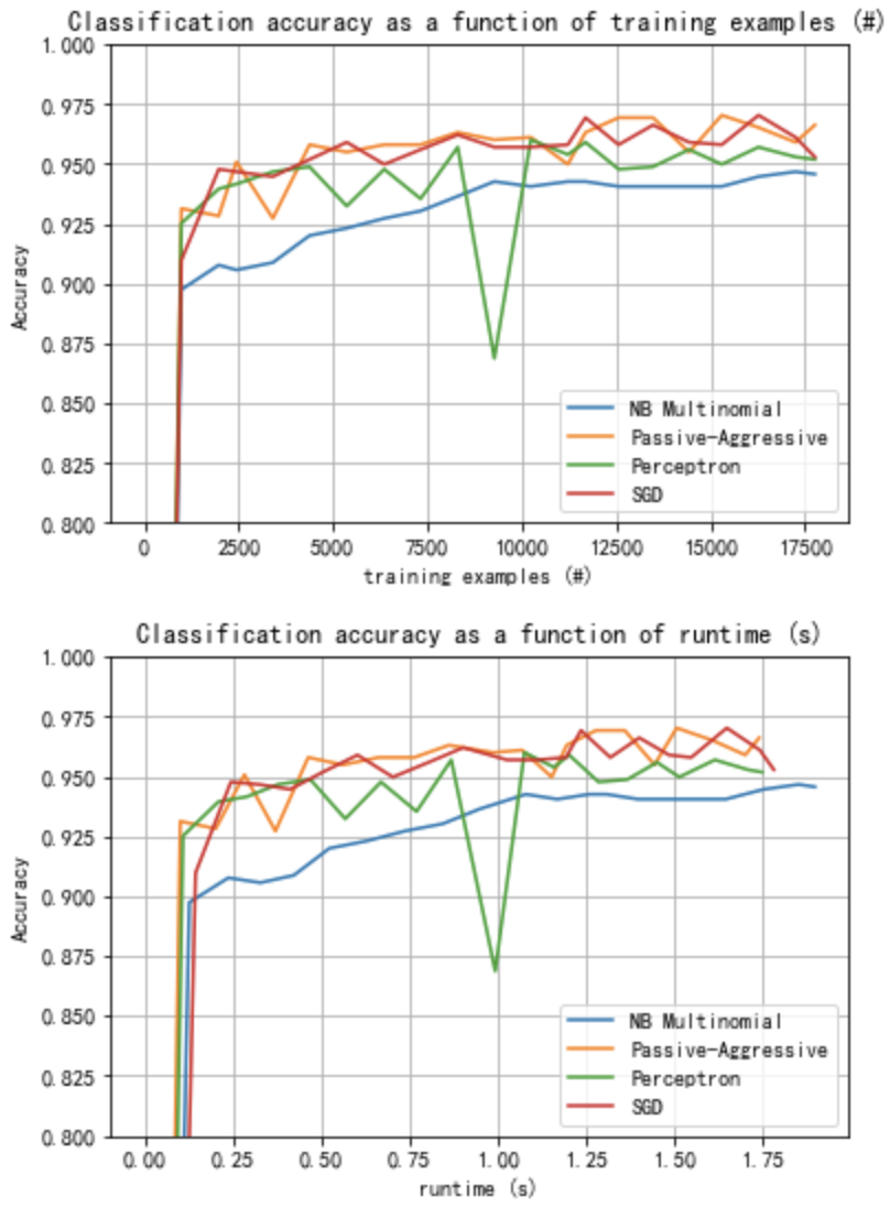
Plot Result
图中表示分类器的学习曲线:分类器的分类精度在批次训练过程中的演变。 在前1000个样本中测量准确性,并将其作为验证集
import matplotlib.pyplot as plt
from matplotlib import rcParams

def plot_accuracy(x, y, x_legend):
    """Plot accuracy as a function of x."""
    x = np.array(x)
    y = np.array(y)
    plt.title('Classification accuracy as a function of %s' % x_legend)
    plt.xlabel('%s' % x_legend)
    plt.ylabel('Accuracy')
    plt.grid(True)
    plt.plot(x, y)


rcParams['legend.fontsize'] = 10
cls_names = list(sorted(cls_stats.keys()))

# Plot accuracy evolution
plt.figure()
for _, stats in sorted(cls_stats.items()):
    # Plot accuracy evolution with #examples
    accuracy, n_examples = zip(*stats['accuracy_history'])
    plot_accuracy(n_examples, accuracy, "training examples (#)")
    ax = plt.gca()
    ax.set_ylim((0.8, 1))
plt.legend(cls_names, loc='best')

plt.figure()
for _, stats in sorted(cls_stats.items()):
    # Plot accuracy evolution with runtime
    accuracy, runtime = zip(*stats['runtime_history'])
    plot_accuracy(runtime, accuracy, 'runtime (s)')
    ax = plt.gca()
    ax.set_ylim((0.8, 1))
plt.legend(cls_names, loc='best')
画出训练时间消耗和对设定的测试数据集进行预测的时间消耗的统计图
# Plot fitting times
plt.figure()
fig = plt.gcf()
cls_runtime = [stats['total_fit_time']
               for cls_name, stats in sorted(cls_stats.items())]

cls_runtime.append(total_vect_time)
cls_names.append('Vectorization')
bar_colors = ['b', 'g', 'r', 'c', 'm', 'y']

ax = plt.subplot(111)
rectangles = plt.bar(range(len(cls_names)), cls_runtime, width=0.5,
                     color=bar_colors)

ax.set_xticks(np.linspace(0, len(cls_names) - 1, len(cls_names)))
ax.set_xticklabels(cls_names, fontsize=10)
ymax = max(cls_runtime) * 1.2
ax.set_ylim((0, ymax))
ax.set_ylabel('runtime (s)')
ax.set_title('Training Times')


def autolabel(rectangles):
    """attach some text vi autolabel on rectangles."""
    for rect in rectangles:
        height = rect.get_height()
        ax.text(rect.get_x() + rect.get_width() / 2.,
                1.05 * height, '%.4f' % height,
                ha='center', va='bottom')
        plt.setp(plt.xticks()[1], rotation=30)


autolabel(rectangles)
plt.tight_layout()
plt.show()

# Plot prediction times
plt.figure()
cls_runtime = []
cls_names = list(sorted(cls_stats.keys()))
for cls_name, stats in sorted(cls_stats.items()):
    cls_runtime.append(stats['prediction_time'])
cls_runtime.append(parsing_time)
cls_names.append('Read/Parse\n+Feat.Extr.')
cls_runtime.append(vectorizing_time)
cls_names.append('Hashing\n+Vect.')

ax = plt.subplot(111)
rectangles = plt.bar(range(len(cls_names)), cls_runtime, width=0.5,
                     color=bar_colors)

ax.set_xticks(np.linspace(0, len(cls_names) - 1, len(cls_names)))
ax.set_xticklabels(cls_names, fontsize=8)
plt.setp(plt.xticks()[1], rotation=30)
ymax = max(cls_runtime) * 1.2
ax.set_ylim((0, ymax))
ax.set_ylabel('runtime (s)')
ax.set_title('Prediction Times (%d instances)' % n_test_documents)
autolabel(rectangles)
plt.tight_layout()
plt.show()


 浙公网安备 33010602011771号