
DoG(difference-of-gaussians)是一个生成边缘图片的算法。最早是Adobe公司的研究员在《XDoG: An eXtended difference-of-Gaussians compendium including advanced image stylization》论文中提出的。作者发现很多论文为了提取边缘不仅仅使用DoG算法,还额外添加了很多复杂的过程。作者认为这些是没有必要的,这些复杂的过程都可以等效为一种DoG。因此作者对DoG进行拓展,发表了这篇XDoG。
DoG使用两个图片的高斯差分图来进行边缘检测。
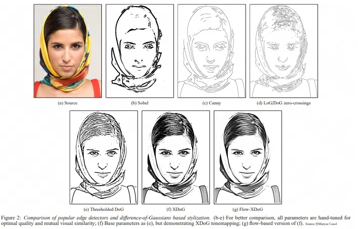
上图是使用不同的方法对原图片(a)处理的结果。
第一行是使用梯度的方法,选取图形梯度为0(或二阶导数)的点组成的边缘图片,可以发现是边缘为线状并且受到噪声影响比较大。
DoG算法流程
- 对于图片Image,设定高斯卷积核的方差sigma和缩放比例k。
- 对图片Image使用高斯滤波器G1进行卷积,得到g1。
- 对图片Image使用高斯滤波器G2进行卷积,得到g2。
- g1-g2得到高斯差分图。
- 取差分图中为0的区域,得到边缘图片。
XDoG改进之处
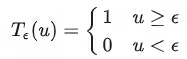
xDoG对DoG中差分图和阈值添加新的参数来控制。
如上图,为了修正边缘处只有一两个像素的问题,使用了阈值的方法去做边缘判定
第二行的(e)是应用阈值处理后的图片,可以发现效果明显比(d)好多了。
参数影响
结合论文方法的代码实现中,会用到sigma、p、epsilon、phi、n_tones等参数,各个参数的作用和取值范围大致如下:
- sigma: 用于图像卷积的高斯核标准差,决定XDoG的空间作用范围。值越大,输出越粗糙抽象,建议常用值约2。
- p: 控制输出锐化程度,值越大可捕捉更细微细节,但会增加对噪声的敏感性,建议范围5-30。
- epsilon: 决定滤波器从常量区间到双曲正切区间的切换阈值,值越大输出越暗且更具戏剧性,建议范围15-65。
- phi: 控制滤波器第二段的斜率特性,值越小会增加灰色渐变层次,负值会反转输出色彩。
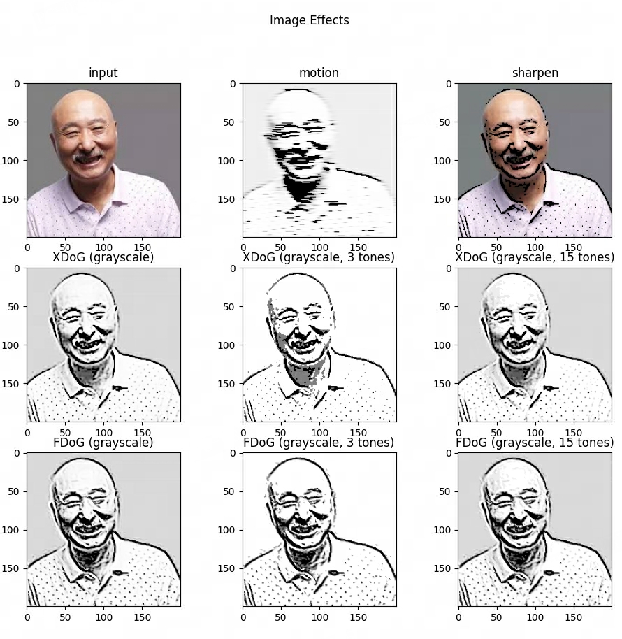
- n_tones: 输出图像的色调分层数。
Flow-DoG改进
此外,若是将高斯差分算子(DoG)扩展成为基于流的高斯差分,把 sigma 用三个独立的参数代替,就变成了基于流的高斯差分Flow-DoG。
- sigma(c):控制用于对图像结构张亮进行高斯模糊的宽度。
- sigma(e):控制沿梯度方向的高斯差分滤波器的宽度。这个值越大,可以得到更多理想的细节,以及更宽的边缘线条。
- sigma(m):控制基于边缘正切值的线积分卷积的宽度。
xDoG核心代码
def xdog_core(I, sigma, p, epsilon, phi, n_tones=None, k = 1.5):
    # Convolve with both standard deviations.
    g1 = gaussian_filter(I, sigma)
    gk = gaussian_filter(I, k * sigma)

    # Rescale phi and epsilon with respect to p.
    phi0 = phi * (p + 1)
    epsilon0 = epsilon / (p + 1)
    tau = p / (p + 1)

    # Compute the difference of gaussians and apply the filter
    D = g1 - tau * gk
    filtered = np.where(D >= epsilon0, 1 + np.tanh(phi0 * (D)), 1)

    # Eventually quantify the tones of the output.
    if n_tones is not None:
        filtered = segmentation(filtered, n_tones, mmin=1, mmax=2)
    out = 255 * normalise(filtered)
    return out
flow-DoG核心代码
def fdog_core(I, sigma_c, sigma_e, sigma_m, sigma_a, p, epsilon, phi, n_tones=None):
    #Compute the edge tangent flow.
    grad_magn0, grad0 = get_gradient(I)
    ETF = get_edge_tangent_flow(flow_iteration(gaussian_filter(I, sigma_c), grad_magn0, grad0))

    #Convolve perpendicularly to edges.
    g1 = convolve_perpendicular(I, ETF, sigma_e)
    gk = convolve_perpendicular(I, ETF, k*sigma_e)

    #Rescale phi and epsilon with respect to p.
    phi0 = phi*(p+1)
    epsilon0 = epsilon/(p+1)
    tau = p/(p+1)

    #Apply the filter.
    D = g1 - tau*gk
    filtered = np.where(D >= epsilon0, 1+np.tanh(phi0*D), 1)

    #Eventually quantify the tones of the output.
    if n_tones is not None:
        filtered = segmentation(filtered, n_tones, mmin=1, mmax=2)

    #Apply two line integral convolutions to increase the coherence of the output.
    O = lic(filtered, np.cos(ETF), np.sin(ETF), sigma_m)
    O = lic(O, np.cos(ETF), np.sin(ETF), sigma_a)
    return normalise(O)*255
实际效果
需要完整代码的朋友,可以站内信或联系邮箱zhyh8341@gmail.com

 浙公网安备 33010602011771号