Linear and Quadratic Programming Solver ( Arithmetic and Algebra) CGAL 4.13 -User Manual
1 Which Programs can be Solved?
This package lets you solve convex quadratic programs of the general form
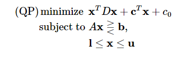
in n real variables x=(x0,…,xn−1).
Here,
- A is an m×n matrix (the constraint matrix),
- b is an m-dimensional vector (the right-hand side),
-
⋛ is an m-dimensional vector of relations from {≤,=,≥},
- l is an n-dimensional vector of lower bounds for x, where lj∈R∪{−∞} for all j
-
u is an n-dimensional vector of upper bounds for x, where uj∈R∪{∞} for all j
-
D is a symmetric positive-semidefinite n×n matrix (the quadratic objective function),
- c is an n-dimensional vector (the linear objective function), and
-
c0 is a constant.
If D=0, the program (QP) is actually a linear program. Section Robustness on robustness briefly discusses the case of D not being positive-semidefinite and therefore not defining a convex program.
Solving the program means to find an n-vector x∗ such that Ax∗⋛b,l≤x∗≤u (a feasible solution), and with the smallest objective function value x∗TDx∗+cTx∗+c0 among all feasible solutions.
There might be no feasible solution at all, in which case the quadratic program is infeasible, or there might be feasible solutions of arbitrarily small objective function value, in which case the program is unbounded.
本包使你能够解决凸二次规划(convex quadratic programs )的通用形式:
其中:x是n个变量的向量,x=x=(x0,…,xn−1)
这里:
- A 是一个mxn矩阵(条件矩阵)。
- b是一个m维的向量(右手边),
-
⋛ 是一个关系 {≤,=,≥}的m维向量,
- l 是一个x的n维下界向量,对于所有j有lj∈R∪{−∞};
-
u 是一个x的n维上界向量 ,对于 所有的j有uj∈R∪{∞};
-
D 是一个对称的半正定的(positive-semidefinite)nxn矩阵(二次型目标函数)
- c 是一个n维向量(线性目标函数)
-
c0 是一个常数.
如果D=0,本规划(QP)实际上是一个线性规划。在Robustness一节,简单讨论了当D不是半正的(positive-semidefinite)而是没有定义一个凸规划情况下的健壮性问题。解这个问题意味着寻找一个n维向量x*,Ax*⋛b,l≤x∗≤u (一个可行解),并且在所有可行解中找到一个最小的目标函数解 x∗TDx∗+cTx∗+c0。
可能根本就没有可行解,这种情况下二次规划为不可行,或可能在可行解中有任意小的目标函数值,即此规划无界。
2 Design, Efficiency, and Robustness
The design of the package is quite simple. The linear or quadratic program to be solved is supplied in form of an object of a class that is a model of the concept QuadraticProgram (or some specialized other concepts, e.g. for linear programs). CGAL provides a number of easy-to-use and flexible models, see Section How to Enter and Solve a Program below. The input data may be of any given number type, such as double, int, or any exact type.
Then the program is solved using the function solve_quadratic_program() (or some specialized other functions, e.g. for linear programs). For this, you also have to provide a suitable exact number type ET used in the solution process. In case of input type double, solution methods that use floating-point-filtering are chosen by default for certain programs (in some cases, this is not appropriate, and the default should be changed; see Section Customizing the Solver for details).
The output of this is an object of Quadratic_program_solution<ET> which you can in turn query for various things: what is the status of the program (optimally solved, infeasible, or unbounded?), what are the values of the optimal solution x∗, what is the associated objective function value, etc.
You can in particular get certificates for the solution. In short, these are proofs that the output is correct. Thus, if you don't believe in the solution (whether it says "optimally solved", "infeasible", or "unbounded"), you can verify it yourself by using the certificates. Section Solution Certificates says more about this.
本包的设计十分简单。线性或二次规划问题求解由一个概念QuadraticProgram (or some specialized other concepts, e.g. for linear programs)的模型类来提供。CGAL提供一个易用的数字和灵活的模型(见How to Enter and Solve a Program小节)。输入的数据可以是任何数据类型,如double,int或任何精确类型。
规划由函数solve_quadratic_program()完成(或其他特殊的函数,即线性规划)。为此,在 你也必须提供一个解过程中使用的合适的精确(exact)数据类型ET。对于输入类型double,使用浮点过滤(floating-point-filtering)解方法将为特定的规划缺省选定(有些情况下,这是不妥的,缺省的方法需要改变,见Customizing the Solver 节)。
解的输出是一个Quadratic_program_solution<ET>对象,你可以通过它得到不同的数据:规划的状态(优化的解、不可行或无界),优化的解x*,相关的目标函数值等。
你可以取得该解的凭据(certificates),即输出正确的证据。如果你不相信这个解,你能自己通过这个凭据验证它(见Solution Certificates节)
2.1 Efficiency
The concept QuadraticProgram (as well as the other specialized ones) require a dense interface of the program, in terms of random-access iterators over the matrices and vectors of (QP). Zero entries therefore play no special role and are treated like all other entries by the interface.
This has mainly historical reasons: the original motivation behind this package was low-dimensional geometric optimization where a dense representation is appropriate and efficient. In fact, the CGAL packages Min_annulus_d<Traits> and Polytope_distance_d<Traits> internally use the linear and quadratic programming solver.
As a user, however, you don't necessarily have to provide a dense representation of your program. You do not pass vectors or matrices to the solution functions, but rather specify the vectors and matrices through iterators. The iterator abstraction easily allows to build models that convert a sparse representation into a dense interface. The predefined models Quadratic_program<NT> and Quadratic_program_from_mps<NT> do exactly this; in using them, you can forget about the dense interface.
Nevertheless, if you care about efficiency, you cannot completely ignore the issue. If you think about a quadratic program in n variables and m constraints, its dense interface has Θ(n2+mn) entries, even if actually very few of them are nonzero. This has consequences for the complexity of the internal computations. In fact, a single iteration of the solution process has complexity at least Ω(mn), since usually, all entries of the matrix A are accessed. This implies that problems where min(n,m) is large cannot be solved efficiently, even if the number of nonzero entries in the problem description is very small.
QuadraticProgram概念(和其他特定的规划)要求一个稠密的接口(dense interface),称为(QP)的矩阵和向量上的随机存取迭代器(random-access iterators over the matrices and vectors of (QP).)。因此0项(entries)被该接口与其他项(entries)同样对待。
这主要是历史原因:本包的设计初衷是在低维的几何优化中一个稠密的表示(dense representation)是合理且高效的。CGAL中Min_annulus_d<Traits>和 Polytope_distance_d<Traits>包内部使用了线性和二次规划解析器。
作为一个用户,你不必要为你的规划提供一个稠密的表示(dense representation)。你不将向量或矩阵传入解函数,但需要通过迭代器来指定向量和矩阵。迭代器抽象容易建立模型,将稀疏表示(sparse representation)转换成稠密表示(dense representation)。预先定义的模型 Quadratic_program<NT> 和 Quadratic_program_from_mps<NT> 就是完成这一过程的。使用它们,你可以不再考虑稠密表示。
但是,如果你对效率很关心。你不能完全忽视这一问题。如果考虑一个n个变量和m个约束条件的二次规划问题,其稠密接口的有 Θ(n2+mn)项,即使其中只有很少项不为0。这将导致复杂的内部运算。实际上,解析过程中单个迭代的复杂度至少为Ω(mn)。因为通常M矩阵所有的项被处理,意味着这个问题将不能被高效地解决(其min(m,n)很大)即使非零项的数量非常小。
We can actually be quite precise about performance, in terms of the following parameters.
- n
- the number of variables (or columns of A),
- m
- the number of constraints (or rows of A)
- e
- the number of equality constraints,
- r
- the rank of the quadratic objective function matrix D.
The time required to solve the problems is in most cases linear in max(n,m), but with a factor heavily depending on min(n,e)+r. Therefore, the solver will be efficient only if min(n,e)+r is small.
Here are the scenarios in which this applies:
- Quadratic programs with a small number of variables, but possibly a large number of inequality constraints,
- Linear programs with a small number of equality constraints but possibly a large number of variables,
- Quadratic programs with a small number of equality constraints and D of small rank, but possibly with a large number of variables.
How small is small? If min(n,e)+r is up to 10, the solver will probably be very fast, even if max(n,m) goes into the millions. If min(n,m)+r is up to a few hundreds, you may still get a solution within reasonable time, depending on the problem characteristics.
If you have a problem where both n and e are well above 1,000, say, then chances are high that CGAL cannot solve it within reasonable time.
我们可以十分准确地调整负荷和表现,通过下列参数:
n : 变量的数量(或矩阵A的列数)
m : 约束的数量 (或A的行数)
e : 等于约束的数量
r : 二次目标函数矩阵D的秩
解决这一问题的时间在大多数情况下是max(m,n)的线性值,但其中一个因子非常依赖于min(n,e)+r。所以,解析器只有在min(n,e)+r小的时候才能高效运行。
下面是可用的场景:
- 小变量规模的二次规划,但也可能用于大数量的不等的约束时。Quadratic programs with a small number of variables, but possibly a large number of inequality constraints,
- 具有小规模的相等约束的但可能具有较多变量的线性规划。Linear programs with a small number of equality constraints but possibly a large number of variables,
- 具有小数量的相等约束并D的秩是小的,但是可能具有大数量的变量。Quadratic programs with a small number of equality constraints and D of small rank, but possibly with a large number of variables.
多少就是我们说的少呢?如果min(n,e)+r 达到了10,解析器将可能会非常快,即使max(n,m)达到了百万。如果min(n,m)+r达到了几百,你仍可能在较理想的时间内完成解,这依赖于问题的特征(problem characteristics)。
如果问题的n和e达到了1000,则CGAL可能会大概率下不能在可期的时间内完成解。
2.2 Robustness
Given that you use an exact number type in the function solve_quadratic_program (or in the other, specialized solution functions), the solver will give you exact rational output, for every convex quadratic program. It may fail to compute a solution only if
- The quadratic program is too large (see the previous subsection on efficiency).
- The quadratic objective function matrix D is not positive-semidefinite (see the discussion below).
- The floating-point filter used by default for certain programs and input type
doublefails due to a double exponent overflow. This happens in rare cases only, and it does not pay off to sacrifice the efficiency of the filtered approach in order to cope with these rare cases. There are means, however, to avoid such problems by switching to a slower non-filtered variant, see Section Exponent Overflow in Double Using Floating-Point Filters. - The solver internally cycles. This also happens in rare cases only. However, if you have a hunch that the solver cycles on your problem, there are means to switch to a slower variant that is guaranteed not to cycle, see Section The Solver Internally Cycles.
The second item merits special attention. First, you may ask why the solver does not check that D is positive semidefinite. But recall that D is given by a dense interface, and it would therefore cost Ω(n2) time already to access all entries of the matrix D. The solver itself gets away with accessing much less entries of D in the relevant case where r, the rank of D, is small.
Nevertheless, the solver contains some runtime checks that may detect that the matrix D is not positive-semidefinite. But you may as well get an "optimal solution" in this case, even with valid certificates. The validity of these certificates, however, depends on D being positive-semidefinite; if this is not the case, the certificates only prove that the solver has found a "critical point" of your (nonconvex) program, but there are no guarantees whatsoever that this is a global optimum, or even a local optimum.
对于每个凸集二次规划,假定你使用一个精确数据类型( exact number type i),函数solve_quadratic_program(或其他特定的解函数)将会给你一个精确的有理输出。可能出现无法得出计算结果的情况只有:
- 二次规模规模太大(见效率节)。
- 二次目标函数矩阵D不是半正定的(见下面讨论)。
- 特点规划使用的缺省浮点过滤器和输入的double类型因double类型的指数而溢出。这种情况很少发生,所以不必要付出降低效率的代价去改变浮点过滤算法。有规避这种情况的方法,即将算法切换到较慢的无过滤模式下(见Exponent Overflow in Double Using Floating-Point Filters)。
- 解析器内部(死)循环。这种情况也不常发生,但如果你直觉解析器出现了循环,则可以通过切换到无过滤模式而避免循环(见The Solver Internally Cycles节)。
第二项需要特别注意。首先,你可以问为什么解析器不去检查D是否为半正定。但前面我们说过,矩阵D是由稠密接口给出的,所以遍历D所有项需要的时间为Ω(n2) ,而解析器本身为了降低运算强度只在矩阵的秩r小时才勉强(gets away with)躲避了处理D中的大量项。但是解析器中仍然有一些运行时检查来判定D是否为半正定的。但这种情况下,你也只是得到一个“优化的解”,即使使用合法的凭据(certificates)。凭据的合法性依赖D是否半正定,如果不是这样的,凭据只能证明解析器找到你的(非凸集)规划的一个“关键点”(“critical point”),它并不能保证全局的最优,甚至也不能保证局部最优。
3 How to Enter and Solve a Program
In this section, we describe how you can supply and solve your problem, using the CGAL program models and solution functions. There are two essentially different ways to proceed, and we will discuss them in turn. In short,
- you can let the model take care of your program data; you start from an empty program and then simply insert the non-zero entries, or read them from a file (more generally, any input stream) in
MPSFormat. You can also change program entries at any time. This is usually the most convenient way if you don't want to care about representation issues; - you can maintain the data yourself and only supply suitable random-access iterators over the matrices and vectors. This is advantageous if you already have the data (explicitly, or implicitly encoded, for example through iterators) and want to avoid copying of data. Typically, this happens if you write generic iterator-based code.
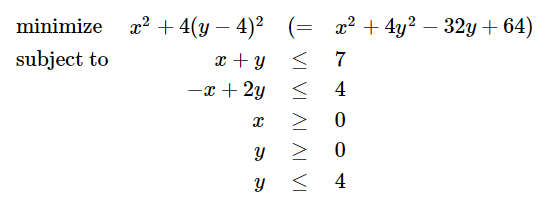
Our running example is the following quadratic program in two variables:
本节描述如何使用CGAL规划模型和解函数呈现并解决问题。有两种不同的方式:
- 你可以让模型来负责你的规划数据,从一个空的规划开始只输入非零项,或从MPSFormat格式文件中读取(也可以是任何流输入)。你也可在任何时候改变规划项。如果你不想关照表示问题,这通常是最方便的方式;
- 你可以自己维护你的数据,只提供矩阵或向量的合适的随机存取迭代器(random-access iterators)。这是非常具有优势的,因为你已经拥有了数据(它们是显式地或隐式地被编码,如通过迭代器)并且不希望复制数据。典型的情况是,如果你写基于通用迭代器的代码时,你正在使用此方法;
Figure 7.1 shows a picture. It depicts the five inequalities of the program, along with the feasible region (green), the set of points that satisfy all the five constraints. The dashed elliptic curves represent contour lines of the objective function, i.e., along each dashed curve, the objective function value is constant.
The global minimum of the objective function is attained at the point (0,4), and the minimum within the feasible region appears at the point (2,3) marked with a black dot. The value of the objective function at this optimal solution is 22+4(3−4)2=8.
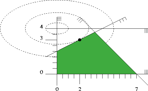
图中显示了可行区域feasible region (green)内5个不等约束条件的规划 。可行区域是满足所有5个约束的点集。虚线椭圆曲线表示目标函数的轮廓线,对于 每条轮廓线目标函数值 是常数。
目标函数的全局最小值在点(0,4)处获得,而在可行区域内则在点(2,3)上取得最小值(黑点表示)。目标函数的最优值是22+4(3−4)2=8。
3.1 Constructing a Program from Data
Here is how this quadratic program can be solved in CGAL according to the first way (letting the model take care of the data). We use int as the input type, and MP_Float or Gmpz (which is faster and preferable if GMP is installed) as the exact type for the internal computations. In larger examples, it pays off to use double as input type in order to profit from the automatic floating-point filtering that takes place then.
For examples how to work with the input type double, we refer to Sections Working from Iterators and Customizing the Solver.
Note: For the quadratic objective function, the entries of the matrix 2D have to be provided, rather than D. Although this is common to almost all quadratic programming solvers, it can easily be overlooked by a novice.
这里介绍第一种解决方法,即让模型来管理数据。我们采用int为输入类型,MP_Float 或 Gmpz为内部计算的精确类型。在更大的例子中,为了得到使用自动浮点过滤器的好处,我们采用double为输入类型,此类例子参见 Working from Iterators 和 Customizing the Solver节。
注意:二次目标函数的矩阵必须是2D,而非D(For the quadratic objective function, the entries of the matrix 2D have to be provided, rather than D),虽然对于 二次规划解析器这是常规,但它很容易被初学者忽视。
If GMP is not installed, the values are of course the same, but numerator and denominator might have a common divisor that is not factored out.
如果GMP没有安装,结果是一样的,但分子和分母可能没有进行约分。
3.2 Constructing a Program from a Stream
Here, the program data must be available in MPSFormat (the MPSFormat page shows how our running example looks like in this format, and it briefly explains the format). Assuming that your working directory contains the file first_qp.mps, the following program will read and solve it, with the same output as before.
这里规划数据必须由MPSFormat格式得到 (MPSFormat节介绍本节例子中的格式)。假定你的工作目录下有一个first_qp.mps,下面的程序将读入并解析它,生成输出。
File QP_solver/first_qp_from_mps.cpp
Note 1: The example shows an interesting feature of this approach: not all data need to come from containers. Here, the iterator over the vector of relations can be provided through the class Const_oneset_iterator<T>, since all entries of this vector are equal to SMALLER. The same could have been done with the vector fl for the finiteness of the lower bounds.
Note 2: The program type looks a bit scary, with its total of 9 template arguments, one for each iterator type. In Section Using Makers we show how the explicit construction of this type can be circumvented.
注意1: 这个方法的有趣之处是:不是所有的数据来自容器。通过类Const_oneset_iterator<T>可以提供关系向量所需的迭代器,因为向量的所有项都与SMALLER相等。对于f1向量下界的有限性做了同样的处理。
注意2: 本规划类型看样子有点唬人,有9个模板参数,每个迭代器类型一个参数。在Using Makers 节我们展示如何绕过(circumvent)这种显式的创建过程。
4 Solving Linear and Nonnegative Programs
Let us reconsider the general form of (QP) from Section Which Programs can be Solved? above. If D=0, the quadratic program is in fact a linear program, and in the case that the bound vectors l is the zero vector and all entries of u are ∞, the program is said to be nonnegative. The package offers dedicated models and solution methods for these special cases.
From an interface perspective, this is just syntactic sugar: in the model Quadratic_program<NT>, we can easily set the default bounds so that a nonnegative program results, and a linear program is obtained by simply not inserting any D-entries. Even in the iterator-based approach (see QP_solver/first_qp_from_iterators.cpp), linear and nonnegative programs can easily be defined through suitable Const_oneset_iterator<T>-style iterators.
The main reason for having dedicated solution methods for linear and nonnegative programs is efficiency: if the solver knows that the program is linear, it can save some computations compared to the general solver that unknowingly has to fiddle around with a zero D-matrix. As in Section Robustness above, we can argue that checking in advance whether D=0 is not an option in general, since this may require Ω(n2) time on the dense interface.
Similarly, if the solver knows that the program is nonnegative, it will be more efficient than under the general bounds l≤x≤u. You can argue that nonnegativity is something that could easily be checked in time O(n)beforehand, but then again nonnegative programs are so frequent that the syntactic sugar aspect becomes somewhat important. After all, we can save four iterators in specifying a nonnegative linear program in terms of the concept NonnegativeLinearProgram rather than LinearProgram.
Often, there are no bounds at all for the variables, i.e., all entries of l are −∞, and all entries of u are ∞ (this is called a free program). There is no dedicated solution method for this case (a free quadratic or linear program is treated like a general quadratic or linear program), but all predefined models make it easy to specify all sorts of default bounds, covering the free case.
NonnegativeLinearProgram 而不使用 LinearProgram。4.1 The Linear Programming Solver
Let's go back to our first quadratic program from above and change it into a linear program by simply removing the quadratic part of the objective function:
线性规划由二次规划转化过来,只需去掉目标函数中的二次项:
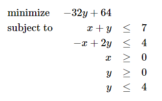
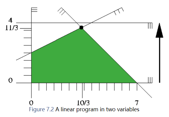
Figure 7.2 shows how this looks like. We will not visualize a linear objective function with contour lines but with arrows instead. The arrow represents the (direction) of the vector −c, and we are looking for a feasible solution that is "extreme" in the direction of the arrow. In our small example, this is the unique point "on" the two constraints x1+x2≤7 and −x1+x2≤4, the point (10/3,11/3) marked with a black dot. The optimal objective function value is −32(11/3)+64=−160/3.
图中给出了线性规划的形态。我们采用一个箭标表示线性目标函数。箭头表示向量−c的(方向),我们正在寻找一个可行的解,这个解在箭头方向上是一个“极值”。在我们的例子中,这个“极值”为图上黑点标识的点,它处于两个约束 x1+x2≤7和−x1+x2≤4的交点 (10/3,11/3) 上。其最优目标函数值是−32(11/3)+64=−160/3。
Here is CGAL code for solving it, using the dedicated LP solver, and according to the three ways for constructing a program that we have already discussed in Section How to Enter and Solve a Program.
QP_solver/first_lp_from_mps.cpp
QP_solver/first_lp_from_iterators.cpp
In all cases, the output is
status: OPTIMAL
objective value: -160/3
variable values:
0: 10/3
1: 11/3
这里是CGAL解的代码,使用了LP解析器,使用了How to Enter and Solve a Program节的三种方法
4.2 The Nonnegative Quadratic Programming Solver
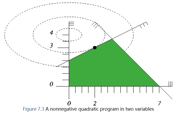
If we go back to our first quadratic program and remove the constraint y≤4, we arrive at a nonnegative quadratic program:
在上面的例子中去除 y≤4,就得到一个非负二次规划。
Figure 7.3 contains the illustration; since the constraint y≤4 was redundant, the feasible region and the optimal solution do not change.
图中显示:因为 y≤4,是冗余的,所以可行区域和最优解没有变化
The following programs (using the dedicated solver for nonnegative quadratic programs) will therefore again output
status: OPTIMAL
objective value: 8/1
variable values:
0: 2/1
1: 3/1
QP_solver/first_nonnegative_qp.cpp
QP_solver/first_nonnegative_qp_from_mps.cpp
QP_solver/first_nonnegative_qp_from_iterators.cpp
4.3 The Nonnegative Linear Programming Solver
Finally, a dedicated model and function is available for nonnnegative linear programs as well. Let's take our linear program from above and remove the constraint y≤4 to obtain a nonnegative linear program. At the same time we remove the constant objective function term to get a "minimal" input and a "shortest" program; the optimal value is −32(11/3)=−352/3.
最后,是专门为非负线性规划提供的模型和函数。本例始于上面的例子并去掉了约束y≤4得到了一个非负线性规划。同时,我们去除目录函数的常数项得到一个“最小”输入和一个“最短”规划,其最优值是−32(11/3)=−352/3
This can be solved by any of the following three programs
QP_solver/first_nonnegative_lp.cpp
QP_solver/first_nonnegative_lp_from_mps.cpp
QP_solver/first_nonnegative_lp_from_iterators.cpp
The output will always be
status: OPTIMAL
objective value: -352/3
variable values:
0: 10/3
1: 11/3
5 Working from Iterators
Here we present a somewhat more advanced example that emphasizes the usefulness of solving linear and quadratic programs from iterators. Let's look at a situation in which a linear program is given implicitly, and access to it is gained through properly constructed iterators.
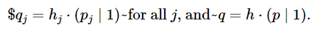
The problem we are going to solve is the following: given points p1,…pn in d-dimensional space and another point p: is p in the convex hull of {p1,…,pn}? In formulas, this is the case if and only if there are real coefficients λ1,…,λn such that p is a convex combination of p1,…,pn:
![]()
The problem of testing the existence of such λj can be expressed as a linear program. It becomes particularly easy when we use the homogeneous representations of the points: if q1,…,qn,q∈Rd+1 are homogeneous coordinates for p1,…,pn,p with positive homogenizing coordinates h1,…,hn,h, we have
Now, nonnegative λ1,…,λn are suitable coefficients for a convex combination if and only if
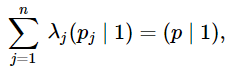
equivalently, if there are μ1,…,μn (with μj=λj⋅h/hj for all j) such that

The linear program now tests for the existence of nonnegative μj that satisfy the latter equation. Below is the code; it defines a function that solves the linear program, given p and p1,…,pn (through an iterator range). The only (mild) trickery involved is the construction of the nested iterator through a fixed column of the constraint matrix A. We get this from transforming the iterator through the points using a functor that maps a point to an iterator through its homogeneous coordinates.
这里我们给出一个更加高级的例子,它强调在解决线性或二次规划时迭代器的作用。当给出兵线性规划是隐含的,并且通过创建合适的迭代器来接入问题。
我们的问题如下:给定d维空间的点集p1,…pn和另一个点p,确定p点是否在{p1,…pn}点集形成的凸包(convex hull)中? 由定理得知,当且仅当存在一个实数系统集λ1,…,λn 使得p是p1,…pn的凸组合
![]()
时本问题成立。
而测试是否存在的问题可以表达为一个线性规划问题。如果q1,…,qn,q∈Rd+1是具有正齐次化坐标h1,…,hn,h的点p1,…,pn,p的齐次坐标,我们使用齐次坐标表示点就十分方便(It becomes particularly easy when we use the homogeneous representations of the points: if q1,…,qn,q∈Rd+1 are homogeneous coordinates for p1,…,pn,p with positive homogenizing coordinates h1,…,hn,h)。我们有:
如果存在一组系数 λ1,…,λn ,当且仅当
时,则 λ1,…,λn 是适合的非负的凸组合系数。
同样地,如果有一组数 μ1,…,μn (对于 所有的j有 μj=λj⋅h/hj ) 满足
现在,线性规划测试满足最后等式的非负的 μj 是否存在,下面是其代码;它定义了一个给定p和p1,…pn(通过iterator给出)解线性规划的函数。这里有点技巧的是通过一个固定列的约束矩阵A创建内嵌的(nested iterator)迭代器。我们通过(We get this from transforming the iterator through the points using a functor that maps a point to an iterator through its homogeneous coordinates)
File QP_solver/solve_convex_hull_containment_lp.h
To see this in action, let us call it with p1=(0,0),p2=(10,0),p3=(0,10) fixed (they define a triangle) and all integral points p in [0,10]2. We know that p is in the convex hull of {p1,p2,p3} if and only if its two coordinates sum up to 10 at most. As the exact type, we use MP_Float or Gmpzf (which is faster and preferable if GMP is installed).
File QP_solver/convex_hull_containment.cpp
5.1 Using Makers
You already noticed in the previous example that the actual template arguments for Nonnegative_linear_program_from_iterators<A_it, B_it, R_it, C_it> can be quite elaborate, and this only gets worse if you plug more iterators into each other. In general, you want to construct a program from given expressions for the iterators, but the types of these expressions are probably very complicated and difficult to look up.
You can avoid the explicit construction of the type Nonnegative_linear_program_from_iterators<A_it, B_it, R_it, C_it> if you only need an expression of it, e.g. to pass it directly as an argument to the solving function. Here is an alternative version of QP_solver/solve_convex_hull_containment_lp.h that shows how this works. In effect, you get shorter and more readable code.
前一个例子中,你已经注意到Nonnegative_linear_program_from_iterators<A_it, B_it, R_it, C_it>的实际模板参数相当复杂。如果你在它们之间插入更多的iterator后。通常,我们想通过一个给定的关于iterator的表达式创建一个规划,但是表达式的类型可能会非常复杂并难以查找。
如果你只需要一个它的表达式,可以通过将它作为参数传递到解析函数就可以避免显式地创建Nonnegative_linear_program_from_iterators<A_it, B_it, R_it, C_it>类型。这里有一个QP_solver/solve_convex_hull_containment_lp.h的替代版本就是展示其方法的。通过这个方法可以得到更加可读的代码。
File QP_solver/solve_convex_hull_containment_lp2.h
6 Important Variables and Constraints
If you have a solution x∗ of a linear or quadratic program, the "important" variables are typically the ones that are not on their bounds. In case of a nonnegative program, these are the nonzero variables. Going back to the example of the previous Section Working from Iterators, we can easily interpret their importance: the nonzero variables correspond to points pj that actually contribute to the convex combination that yields p.
The following example shows how we can access the important variables, using the iterators basic_variable_indices_begin() and basic_variable_indices_end().
We generate a set of points that form a 4-gon in [0,4]2, and then find the ones that contribute to the convex combinations of all 25 lattice points in [0,4]2. If the lattice point in question is not in the 4-gon, we simply output this fact.
如果你有线性或二次规划的一个解x∗,“重要的”变量是哪些典型地在边界之外的变量。在非负规划的情况,有非零变量。在Working from Iterators节的例子中,我们可以容易解释它们的重要性:非零变量与生成关于p的凸组合做出实际贡献的pj对应。(Going back to the example of the previous Section Working from Iterators, we can easily interpret their importance: the nonzero variables correspond to points pj that actually contribute to the convex combination that yields p)
File QP_solver/important_variables.cpp
It turns out that exactly three of the four points contribute to any convex combination, even through there are lattice points that lie in the convex hull of less than three of the points. This shows that the set of basic variables that we access in the example does not necessarily coincide with the set of important variables as defined above. In fact, it is only guaranteed that a non-basic variable attains one of its bounds, but there might be basic variables that also have this property. In linear and quadratic programming terms, such a situation is called a degeneracy.
There is also the concept of an important constraint: this is typically a constraint in the system Ax⋛b that is satisfied with equality at x∗. Program QP_solver/first_qp_basic_constraints.cpp shows how these can be accessed, using the iterators basic_constraint_indices_begin() and basic_constraint_indices_end().
Again, we have a disagreement between "basic" and "important": it is guaranteed that all basic constraints are satisfied with equality at x∗, but there might be non-basic constraints that are satisfied with equality as well.
结果是四个点中的三个对任意 凸组合有贡献,即使存在格点处于少于3个点的凸包内(even through there are lattice points that lie in the convex hull of less than three of the points)。
7 Solution Certificates
Suppose the solver tells you that the problem you have entered is infeasible. Why should you believe this? Similarly, you can quite easily verify that a claimed optimal solution is feasible, but why is there no better one?
Certificates are proofs that the solver can give you in order to convince you that what it claims is indeed true. The archetype of such a proof is Farkas Lemma [1].
Farkas Lemma: Either the inequality system
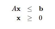
has a solution x∗, or there exists a vector y such that
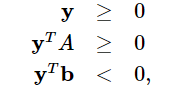
but not both.
Thus, if someone wants to convince you that the first system in the Farkas Lemma is infeasible, that person can simply give you a vector y that solves the second system. Since you can easily verify yourself that the y you got satisfies this second system, you now have a certificate for the infeasibility of the first system, assuming that you believe in Farkas Lemma.
Here we show how the solver can convince you. We first set up an infeasible linear program with constraints of the type Ax≤b,x≥0; then we solve it and ask for a certificate. Finally, we verify the certificate by simply checking the inequalities of the second system in Farkas Lemma.
File QP_solver/infeasibility_certificate.cpp
There are similar certificates for optimality and unboundedness that you can see in action in the programs QP_solver/optimality_certificate.cpp and QP_solver/unboundedness_certificate.cpp. The underlying variants of Farkas Lemma are somewhat more complicated, due to the mixed relations in ⋛ and the general bounds. The certificate section of Quadratic_program_solution<ET> gives the full picture and mathematically proves the correctness of the certificates.
8 Customizing the Solver
Sometimes it is necessary to alter the default behavior of the solver. This can be done by passing a suitably prepared object of the class Quadratic_program_options to the solution functions. Most options concern "soft" issues like verbosity, but there are two notable case where it is of critical importance to be able to change the defaults.
8.1 Exponent Overflow in Double Using Floating-Point Filters
The filtered version of the solver that is used for some problems by default on input type double internally constructs double-approximations of exact multiprecision values. If these exact values are extremely large, this may lead to infinite double values and incorrect results. In debug mode, the solver will notice this through a certificate cross-check in the end (or even earlier). In this case, it is advisable to explicitly switch to a non-filtered pricing strategy, see Quadratic_program_pricing_strategy.
Hint: If you have a program where the number of variables n and the number of constraints m have the same order of magnitude, the filtering will usually have no dramatic effect on the performance, so in that case you might as well switch to QP_PARTIAL_DANTZIG to be safe from the issue described here (see QP_solver/cycling.cpp for an example that shows how to change the pricing strategy).
8.2 The Solver Internally Cycles
Consider the following program. It reads a nonnegative linear program from the file cycling.mps (which is in the example directory as well), and then solves it in verbose mode, using Bland's rule, see Quadratic_program_pricing_strategy.
File QP_solver/cycling.cpp
If you comment the line
options.set_pricing_strategy(CGAL::QP_BLAND); // Bland's rule
you will see that the solver cycles: the verbose mode outputs the same sequence of six iterations over and over again. By switching to QP_BLAND, the solution process typically slows down a bit (it may also speed up in some cases), but now it is guaranteed that no cycling occurs.
In general, the verbose mode can be of use when you are not sure whether the solver "has died", or whether it simply takes very long to solve your problem. We refer to the class Quadratic_program_options for further details.
9 Some Benchmarks for Convex Hull Containment
Here we want to show what you can expect from the solver's performance in a specific application; we don't know whether this application is typical in your case, and we make no claims whatsoever about the performance in other applications.
Still, the example shows that the performance can be dramatically affected by switching between pricing strategies, and we give some hints on how to achieve good performance in general.
The application is the one already discussed in Section Working from Iterators above: testing whether a point is in the convex hull of other points. To be able to switch between pricing strategies, we add another parameter of type Quadratic_program_options to the function solve_convex_hull_containment_lp that we pass on to the solution function:
File QP_solver/solve_convex_hull_containment_lp3.h
Now let us test containment of the origin in the convex hull of n random points in [0,1]d (it will most likely not be contained, and it turns out that this is the most expensive case). In the program below, we use d=10 and n=100,000, and we comment on some other combinations of n and d below (feel free to experiment with still other values).
File QP_solver/convex_hull_containment_benchmarks.cpp
If you compile with the macros NDEBUG or CGAL_QP_NO_ASSERTIONS set (this is essential for good performance!!), you will see runtimes that qualitatively look as follows (on your machine, the actual runtimes will roughly be some fixed multiples of the numbers in the table below, and they might vary with the random choices). The default choice of the pricing strategy in that case is QP_PARTIAL_FILTERED_DANTZIG.
| Strategy | Runtime in seconds |
|---|---|
QP_CHOOSE_DEFAULT |
0.32 |
QP_DANTZIG |
10.7 |
QP_PARTIAL_DANTZIG |
3.72 |
QP_BLAND |
3.65 |
QP_FILTERED_DANTZIG |
0.43 |
QP_PARTIAL_FILTERED_DANTZIG |
0.32 |
We clearly see the effect of filtering: we gain a factor of ten, roughly, compared to the next best non-filtered variant.
9.1 d=3, n=1,000,000
The filtering effect is amplified if the points/dimension ratio becomes larger. This is what you might see in dimension three, with one million points.
| Strategy | Runtime in seconds |
|---|---|
QP_CHOOSE_DEFAULT |
1.34 |
QP_DANTZIG |
47.6 |
QP_PARTIAL_DANTZIG |
15.6 |
QP_BLAND |
16.02 |
QP_FILTERED_DANTZIG |
1.89 |
QP_PARTIAL_FILTERED_DANTZIG |
1.34 |
In general, if your problem has a high variable/constraint or constraint/variable ratio, then filtering will typically pay off. In such cases, it might be beneficial to encode your problem using input type double in order to profit from the filtering (but see the issue discussed in Section Exponent Overflow in Double Using Floating-Point Filters).
9.2 d=100, n=100,000
Conversely, the filtering effect deteriorates if the points/dimension ratio becomes smaller.
| Strategy | Runtime in seconds |
|---|---|
QP_CHOOSE_DEFAULT |
3.05 |
QP_DANTZIG |
78.4 |
QP_PARTIAL_DANTZIG |
45.9 |
QP_BLAND |
33.2 |
QP_FILTERED_DANTZIG |
3.36 |
QP_PARTIAL_FILTERED_DANTZIG |
3.06 |
9.3 d=500, n=1,000
If the points/dimension ratio tends to a constant, filtering is no longer a clear winner. The reason is that in this case, the necessary exact calculations with multiprecision numbers dominate the overall runtime.
| Strategy | Runtime in seconds |
|---|---|
QP_CHOOSE_DEFAULT |
2.65 |
QP_DANTZIG |
5.55 |
QP_PARTIAL_DANTZIG |
5.6 |
QP_BLAND |
4.46 |
QP_FILTERED_DANTZIG |
2.65 |
QP_PARTIAL_FILTERED_DANTZIG |
2.61 |
In general, if you have a program where the number of variables and the number of constraints have the same order of magnitude, then the saving gained from using the filtered approach is typically small. In such a situation, you should consider switching to a non-filtered variant in order to avoid the rare issue discussed in Section Exponent Overflow in Double Using Floating-Point Filters altogether.

 浙公网安备 33010602011771号