Abstract
The dominant sequence transduction models are based on complex recurrent or convolutional neural networks that include an encoder and a decoder. The best performing models also connect the encoder and decoder through an attention mechanism. We propose a new simple network architecture, the Transformer, based solely on attention mechanisms, dispensing with recurrence and convolutions entirely. Experiments on two machine translation tasks show these models to be superior in quality while being more parallelizable and requiring significantly less time to train. Our model achieves 28.4 BLEU on the WMT 2014 Englishto-German translation task, improving over the existing best results, including ensembles, by over 2 BLEU. On the WMT 2014 English-to-French translation task, our model establishes a new single-model state-of-the-art BLEU score of 41.8 after training for 3.5 days on eight GPUs, a small fraction of the training costs of the best models from the literature. We show that the Transformer generalizes well to other tasks by applying it successfully to English constituency parsing both with large and limited training data.
主要的序列转换任务是基于复杂的循环或者卷积神经网络包括一个编码器和解码器。最好表现的模型通过一个注意机制连接编码器和解码器。我们采用了一个新的简单的网络架构,Transformer,仅基于注意机制,完全抛弃循环和卷积。在两个机器翻译的任务上显示这些模型质量要更优同时更加并行化和需要更少的时间进行训练。我们的模型实现了28.4BLEU 在WMT2014Englishto-German翻译任务中,超过了现有的最好的结果,包括集合体,超过了2个BLEU。WMT2014English-to-French 翻译任务中,在8块GPU上训练了3.5天后,我们建立了一个简单的模型最先进的BLEU得分为41.8, 这只是文献中最有模型的一小部分训练成本。通过成功将transformer应用到大量和有限的数据样本的英文选区任务,我们显示了transformer可以很好的推广到其他任务上
Introduction
Recurrent neural networks, long short-term memory [13] and gated recurrent [7] neural networks in particular, have been firmly established as state of the art approaches in sequence modeling and transduction problems such as language modeling and machine translation [35, 2, 5]. Numerous efforts have since continued to push the boundaries of recurrent language models and encoder-decoder architectures [38, 24, 15].
循环神经网络,特别是长短时记忆和门控递归神经网络,已经稳固的被确定时最好的方法在序列模型和转换任务比如语言模型和机器翻译。从那以后,无数的努力持续的推进循环模型和编解码器结构的边界
Recurrent models typically factor computation along the symbol positions of the input and output sequences. Aligning the positions to steps in computation time, they generate a sequence of hidden states ht, as a function of the previous hidden state ht−1 and the input for position t. This inherently sequential nature precludes parallelization within training examples, which becomes critical at longer sequence lengths, as memory constraints limit batching across examples. Recent work has achieved significant improvements in computational efficiency through factorization tricks [21] and conditional computation [32], while also improving model performance in case of the latter. The fundamental constraint of sequential computation, however, remains.
循环模型通过输入和输出序列的符号位置进行因子计算。在计算时间内将位置和步数对齐,他们生成一系列隐藏层,作为先前隐藏层ht-1和输入位置t的函数。这种固有的序列结构排除了训练样本的并引化,在较长序列上的长度变得至关重要,因为内存约束限制了跨示例的批处理。最近的工作通过分解技巧和条件计算实现了一个重要的改进,同时在最新的例子种也改善了模型的效果。然而顺序计算的基本约束仍然存在
Attention mechanisms have become an integral part of compelling sequence modeling and transduction models in various tasks, allowing modeling of dependencies without regard to their distance in the input or output sequences [2, 19]. In all but a few cases [27], however, such attention mechanisms are used in conjunction with a recurrent network.
注意机制已经称为引人瞩目的各种序列模型和转导模型的重要组成部分,允许对依赖关系建模而不需要考虑输入和输出序列的长度。然后在少数任务种,注意机制也于循环网络结合使用
In this work we propose the Transformer, a model architecture eschewing recurrence and instead relying entirely on an attention mechanism to draw global dependencies between input and output. The Transformer allows for significantly more parallelization and can reach a new state of the art in translation quality after being trained for as little as twelve hours on eight P100 GPUs.
在这个任务种我们使用Transformer,一个模型结构避开循环和完全依赖注意机制去吸引输入和输出之间的全局依赖。Transformer允许更多的并行化和在8块P100的GPU上训练12个小时可以在翻译中达到一个好的质量。
Model Architecture

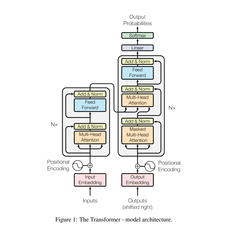
Most competitive neural sequence transduction models have an encoder-decoder structure [5, 2, 35]. Here, the encoder maps an input sequence of symbol representations (x1, ..., xn) to a sequence of continuous representations z = (z1, ..., zn). Given z, the decoder then generates an output sequence (y1, ..., ym) of symbols one element at a time. At each step the model is auto-regressive [10], consuming the previously generated symbols as additional input when generating the next. The Transformer follows this overall architecture using stacked self-attention and point-wise, fully connected layers for both the encoder and decoder, shown in the left and right halves of Figure 1, respectively
最具竞争力的神经转导序列模型有一个编解码结构。这里,编码器映射一个输入序列(x1, ..., xn)符号表示一个持续的序列表示Z=(z1,.....zn).给出的Z,这个解码器生成一个输出序列(y1,....,ym)每次一个元素的符号。在每一步中,模型都是自回归的,当生成下一个时,评估之前生成的符号作为另外的输入。Transformer准许这个整体的架构使用堆叠自我注意和点式,全连接层对于整个编码器和解码器,将分别展示在图一中的左和右两个部分
3.1 Encoder and Decoder Stacks
Encoder: The encoder is composed of a stack of N = 6 identical layers. Each layer has two sub-layers. The first is a multi-head self-attention mechanism, and the second is a simple, positionwise fully connected feed-forward network. We employ a residual connection [11] around each of the two sub-layers, followed by layer normalization [1]. That is, the output of each sub-layer is LayerNorm(x + Sublayer(x)), where Sublayer(x) is the function implemented by the sub-layer itself. To facilitate these residual connections, all sub-layers in the model, as well as the embedding layers, produce outputs of dimension dmodel = 512.
编码器: 这个编码器有6个完全相同的层堆叠而成。每一个层有两个子层。第一个是一个多头的自注意机制,第二个是一个简单的,全连接的feed-forward网络,我们在这两个子层周围使用残差连接,后面跟着一个层归一化。每一个子层的输出是LayerNorm(x + Sublayer(x)),其中子层是由子层自身实现的功能。为了促进残差的连接,在模型中的所有子层和隐藏层,提供一个模型尺寸512的输出
Encoder的代码
class Encoder(nn.Module):
    """多层EncoderLayer组成Encoder。"""

    def __init__(self,
               vocab_size,
               max_seq_len,
               num_layers=6,
               model_dim=512,
               num_heads=8,
               ffn_dim=2048,
               dropout=0.0):
        super(Encoder, self).__init__()

        self.encoder_layers = nn.ModuleList(
          [EncoderLayer(model_dim, num_heads, ffn_dim, dropout) for _ in
           range(num_layers)])

        self.seq_embedding = nn.Embedding(vocab_size + 1, model_dim, padding_idx=0)
        self.pos_embedding = PositionalEncoding(model_dim, max_seq_len)

    def forward(self, inputs, inputs_len):
        output = self.seq_embedding(inputs)  # 对输入求取embedding
        output += self.pos_embedding(inputs_len) # 对位置做embedding

        self_attention_mask = padding_mask(inputs, inputs) # 生成全零的B L L mask
attentions = []
for encoder in self.encoder_layers:
output, attention = encoder(output, self_attention_mask)
attentions.append(attention)
return output, attentions
上面使用到的EncoderLayer的代码
class EncoderLayer(nn.Module):
    """Encoder的一层。"""

    def __init__(self, model_dim=512, num_heads=8, ffn_dim=2048, dropout=0.0):
        super(EncoderLayer, self).__init__()

        self.attention = MultiHeadAttention(model_dim, num_heads, dropout)
        self.feed_forward = PositionalWiseFeedForward(model_dim, ffn_dim, dropout)

    def forward(self, inputs, attn_mask=None):

        # self attention
        context, attention = self.attention(inputs, inputs, inputs, padding_mask)

        # feed forward network
        output = self.feed_forward(context)

        return output, attention
Decoder: The decoder is also composed of a stack of N = 6 identical layers. In addition to the two sub-layers in each encoder layer, the decoder inserts a third sub-layer, which performs multi-head attention over the output of the encoder stack. Similar to the encoder, we employ residual connections around each of the sub-layers, followed by layer normalization. We also modify the self-attention sub-layer in the decoder stack to prevent positions from attending to subsequent positions. This masking, combined with fact that the output embeddings are offset by one position, ensures that the predictions for position i can depend only on the known outputs at positions less than i.
解码器: 解码器同样也是有6个相同的堆叠层构成。另外两个子层在每个解码器中,解码器插入了一个第三个子层,对编码器的堆叠的输出实现多头注意。与编码器相同的,我们在每一个子层的周围采用残差连接,后面跟层归一化。我们也修改自注意子层在解码器的堆叠层,防止一个位置注意到下一个位置。这种掩饰,加上输出嵌入被偏移一个像素的事实,确定对于位置i的输出仅依赖已经的输出位置小于i
Decoder的代码
class Decoder(nn.Module):

    def __init__(self,
               vocab_size,
               max_seq_len,
               num_layers=6,
               model_dim=512,
               num_heads=8,
               ffn_dim=2048,
               dropout=0.0):
        super(Decoder, self).__init__()

        self.num_layers = num_layers

        self.decoder_layers = nn.ModuleList(
          [DecoderLayer(model_dim, num_heads, ffn_dim, dropout) for _ in
           range(num_layers)])

        self.seq_embedding = nn.Embedding(vocab_size + 1, model_dim, padding_idx=0)
        self.pos_embedding = PositionalEncoding(model_dim, max_seq_len)

    def forward(self, inputs, inputs_len, enc_output, context_attn_mask=None):
        output = self.seq_embedding(inputs) # 输入嵌入
        output += self.pos_embedding(inputs_len) # 位置嵌入

        self_attention_padding_mask = padding_mask(inputs, inputs) # 对输入做补零操作
        seq_mask = sequence_mask(inputs) #输入的特征掩码,使得当前特征只能看到之前的特征
self_attn_mask = torch.gt((self_attention_padding_mask + seq_mask), 0) #大于0的位置显示1
self_attentions = []
context_attentions = []
for decoder in self.decoder_layers:
output, self_attn, context_attn = decoder(
output, enc_output, self_attn_mask, context_attn_mask)
self_attentions.append(self_attn)
context_attentions.append(context_attn)
return output, self_attentions, context_attentions
上面的Sequnce_mask的代码
def sequence_mask(seq):
    batch_size, seq_len = seq.size()
    mask = torch.triu(torch.ones((seq_len, seq_len), dtype=torch.uint8),
                    diagonal=1) #主对角上向下一个位置是1,其他位置是0 [0 1 1
                                                               # 0 0 1
                                                               # 0 0 0]
    mask = mask.unsqueeze(0).expand(batch_size, -1, -1)  # [B, L, L]
    return mask

上面DecoderLayer的代码, 相比与EncoderLayer,这里多了一个多头注意机制模块,用来对之后输入做掩码隐藏
class DecoderLayer(nn.Module):

    def __init__(self, model_dim, num_heads=8, ffn_dim=2048, dropout=0.0):
        super(DecoderLayer, self).__init__()

        self.attention = MultiHeadAttention(model_dim, num_heads, dropout)
        self.feed_forward = PositionalWiseFeedForward(model_dim, ffn_dim, dropout)

    def forward(self,
              dec_inputs,
              enc_outputs,
              self_attn_mask=None,
              context_attn_mask=None):
        # self attention, all inputs are decoder inputs
        dec_output, self_attention = self.attention(
          dec_inputs, dec_inputs, dec_inputs, self_attn_mask)

        # context attention
        # query is decoder's outputs, key and value are encoder's inputs
        dec_output, context_attention = self.attention(
          enc_outputs, enc_outputs, dec_output, context_attn_mask)

        # decoder's output, or context
        dec_output = self.feed_forward(dec_output)

        return dec_output,
3.2 Attention
An attention function can be described as mapping a query and a set of key-value pairs to an output, where the query, keys, values, and output are all vectors. The output is computed as a weighted sum of the values, where the weight assigned to each value is computed by a compatibility function of the query with the corresponding key.
注意机制可以被描述为映射一个查询和一系列对于输出的键值对,查询,键,值和输出都是向量。输出是作为值的加权和的计算,分配给每一个值的权重是通过一个兼容查询功能和对应键计算获得的
3.2.1 Scaled Dot-Product Attention
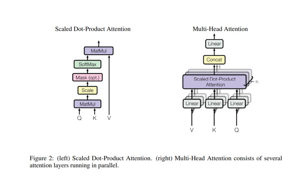
We call our particular attention "Scaled Dot-Product Attention" (Figure 2). The input consists of queries and keys of dimension dk, and values of dimension dv. We compute the dot products of the query with all keys, divide each by √ dk, and apply a softmax function to obtain the weights on the values. In practice, we compute the attention function on a set of queries simultaneously, packed together into a matrix Q. The keys and values are also packed together into matrices K and V . We compute the matrix of outputs as:
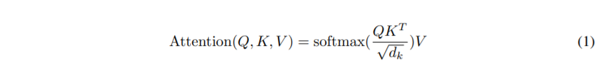
我们叫我们特别的注意 "按比例缩小的点积注意"。这个输入包含问题和维度的键dk和维度的值dv。我们计算查询与所有键的点积,每个被√ dk除,采用一个softmax函数去获得值的权重。在练习中,我们计算注意功能在一系列相似的问题,打包成矩形Q,这些键和值同意被打包成矩形K和V,我们计算输出的矩形如
The two most commonly used attention functions are additive attention [2], and dot-product (multiplicative) attention. Dot-product attention is identical to our algorithm, except for the scaling factor of √ 1 dk . Additive attention computes the compatibility function using a feed-forward network with a single hidden layer. While the two are similar in theoretical complexity, dot-product attention is much faster and more space-efficient in practice, since it can be implemented using highly optimized matrix multiplication code
两种最常见的注意力功能是附加注意力和点乘注意力。点乘注意力和我们的算法是一样的,除了一个√ 1 dk缩放因子。附加注意力使用一个带简单隐藏层的前向网络计算兼容性函数。虽然两者在理论复杂性是一致的,在实际中,点乘注意机制更快并且空间上更有效,因此它可以实现使用高度优化的矩形乘法代码
While for small values of dk the two mechanisms perform similarly, additive attention outperforms dot product attention without scaling for larger values of dk [3]. We suspect that for large values of dk, the dot products grow large in magnitude, pushing the softmax function into regions where it has extremely small gradients 4 . To counteract this effect, we scale the dot products by √ 1 dk .
然而当dk很小的时候,两种结果表现是一致的,当dk的值增大时,加注意机制优于点积的注意。我们认为对于大的dk值,点积的量变大,使得推动softmax函数向梯度极小的区域移动,为了避免这种影响,我们将点积进行√ 1 dk缩放
class ScaledDotProductAttention(nn.Module):
    """Scaled dot-product attention mechanism."""

    def __init__(self, attention_dropout=0.0):
        super(ScaledDotProductAttention, self).__init__()
        self.dropout = nn.Dropout(attention_dropout)
        self.softmax = nn.Softmax(dim=2)

    def forward(self, q, k, v, scale=None, attn_mask=None):
        """
        前向传播.
        Args:
            q: Queries张量,形状为[B, L_q, D_q]
            k: Keys张量,形状为[B, L_k, D_k]
            v: Values张量,形状为[B, L_v, D_v],一般来说就是k
            scale: 缩放因子,一个浮点标量
            attn_mask: Masking张量,形状为[B, L_q, L_k]

        Returns:
            上下文张量和attention张量
        """
        attention = torch.bmm(q, k.transpose(1, 2))
        if scale:
            attention = attention * scale
        if attn_mask:
            # 给需要mask的地方设置一个负无穷
            attention = attention.masked_fill_(attn_mask, -np.inf)
        # 计算softmax
        attention = self.softmax(attention)
        # 添加dropout
attention = self.dropout(attention)
# 和V做点积
context = torch.bmm(attention, v)
return context, attention
3.2.2 Multi-Head Attention
Instead of performing a single attention function with dmodel-dimensional keys, values and queries, we found it beneficial to linearly project the queries, keys and values h times with different, learned linear projections to dk, dk and dv dimensions, respectively. On each of these projected versions of queries, keys and values we then perform the attention function in parallel, yielding dv-dimensional output values. These are concatenated and once again projected, resulting in the final values, as depicted in Figure 2.
而不是使用dmodel维度的键,值,问题的单一注意功能,我们发现,将查询和键,值以不同的方式线性投影h次是有益的,分别学习了dk,dk和dv维度的线性投影。在每一个查询投影版本上, 键和值我们同时执行注意机制,生成dv维度的输出值。这些被连接并进行再次投射,造成的最终的值,在图2中被显示
Multi-head attention allows the model to jointly attend to information from different representation subspaces at different positions. With a single attention head, averaging inhibits this.

多头注意使得模型能在不同的位置共同关注来自不同子模块的信息。只用一个简单的注意头,将平均抑制这种情况
Where the projections are parameter matrices W Q i ∈ R dmodel×dk , W K i ∈ R dmodel×dk , WV i ∈ R dmodel×dv and WO ∈ R hdv×dmodel . In this work we employ h = 8 parallel attention layers, or heads. For each of these we use dk = dv = dmodel/h = 64. Due to the reduced dimension of each head, the total computational cost is similar to that of single-head attention with full dimensionality.
其中投影为参数矩阵WQ, WK和WV和WO。在这个工作中我们采用8个平行注意层或者头。对于每一个这些,我们使用dk=dv=dmodel/h = 64表示。由于减少了每个头的尺寸,总的消耗与单个头注意的全维度的相似。
Multi-Head Attention代码
class MultiHeadAttention(nn.Module):

    def __init__(self, model_dim=512, num_heads=8, dropout=0.0):
        super(MultiHeadAttention, self).__init__()

        self.dim_per_head = model_dim // num_heads
        self.num_heads = num_heads
        self.linear_k = nn.Linear(model_dim, self.dim_per_head * num_heads)
        self.linear_v = nn.Linear(model_dim, self.dim_per_head * num_heads)
        self.linear_q = nn.Linear(model_dim, self.dim_per_head * num_heads)

        self.dot_product_attention = ScaledDotProductAttention(dropout)
        self.linear_final = nn.Linear(model_dim, model_dim)
        self.dropout = nn.Dropout(dropout)

        # multi-head attention之后需要做layer norm
        self.layer_norm = nn.LayerNorm(model_dim)

    def forward(self, key, value, query, attn_mask=None):
        # 残差连接
        residual = query
        dim_per_head = self.dim_per_head
        num_heads = self.num_heads
        batch_size = key.size(0)

        # linear project
         key = self.linear_k(key)
        value = self.linear_v(value)
        query = self.linear_q(query)

        # split by heads
        key = key.view(batch_size * num_heads, -1, dim_per_head) # 拆分成多个头
        value = value.view(batch_size * num_heads, -1, dim_per_head)
        query = query.view(batch_size * num_heads, -1, dim_per_head)

        if attn_mask:
            attn_mask = attn_mask.repeat(num_heads, 1, 1)

        # scaled dot product attention
        scale = (key.size(-1)) ** -0.5
        context, attention = self.dot_product_attention(
            query, key, value, scale, attn_mask)

        # concat heads
        context = context.view(batch_size, -1, dim_per_head * num_heads) # 重新组合

        # final linear projection
        output = self.linear_final(context)

        # dropout
        output = self.dropout(output)

        # add residual and norm layer
        output = self.layer_norm(residual + output)

        return output, attention
3.2.3 Applications of Attention in our Model
The Transformer uses multi-head attention in three different ways:
In "encoder-decoder attention" layers, the queries come from the previous decoder layer, and the memory keys and values come from the output of the encoder. This allows every position in the decoder to attend over all positions in the input sequence. This mimics the typical encoder-decoder attention mechanisms in sequence-to-sequence models such as [38, 2, 9].
Transformer使用多头注意机制在3个不同方面:
在编码和解码注意层,询问来自于上一个与之前的解码层,并且记忆的键和值来自于编码器的输出。这使得编码器每一个位置可以参加输入序列的每一个位置。这模仿编码器和解码器的注意机制在序列对序列模型中。
The encoder contains self-attention layers. In a self-attention layer all of the keys, values and queries come from the same place, in this case, the output of the previous layer in the encoder. Each position in the encoder can attend to all positions in the previous layer of the encoder.
这个编码器包含自注意层。在自注意层的键,值和询问来自于相同的地方,在这个例子中,是编码器前一层的输出。编码器上每一个位置都可以对应上编码器中上一个层的位置。
Similarly, self-attention layers in the decoder allow each position in the decoder to attend to all positions in the decoder up to and including that position. We need to prevent leftward information flow in the decoder to preserve the auto-regressive property. We implement this inside of scaled dot-product attention by masking out (setting to −∞) all values in the input of the softmax which correspond to illegal connections. See Figure 2.
相似的,自注意层在解码器中解码器的每一个位置关注解码器中的任意位置包括其自身。我们需要防止解码器的信息向左流动,保证自回归的准确性。我们通过屏蔽设置(setting to −∞)softmax输入对所有非法的连接缩放点乘注意。
3.3 Position-wise Feed-Forward Networks
In addition to attention sub-layers, each of the layers in our encoder and decoder contains a fully connected feed-forward network, which is applied to each position separately and identically. This consists of two linear transformations with a ReLU activation in between.

除了注意子层,在我们每一层的编码器和解码器都包含全连接的前向网络,它分别和相同应用在每一个位置,在这包含两个线性transformations之间包含Relu激活层
While the linear transformations are the same across different positions, they use different parameters from layer to layer. Another way of describing this is as two convolutions with kernel size 1. The dimensionality of input and output is dmodel = 512, and the inner-layer has dimensionality df f = 2048.
不同位置的线性变化是相同的,在层与层之间,他们使用不同的参数。另外一个方法描述这两个卷积使用1的核尺寸。输入和输出的维度是512,内部层的尺寸是2048
class PositionalWiseFeedForward(nn.Module):

    def __init__(self, model_dim=512, ffn_dim=2048, dropout=0.0):
        super(PositionalWiseFeedForward, self).__init__()
        self.w1 = nn.Conv1d(model_dim, ffn_dim, 1)
        self.w2 = nn.Conv1d(ffn_dim, model_dim, 1)
        self.dropout = nn.Dropout(dropout)
        self.layer_norm = nn.LayerNorm(model_dim)

    def forward(self, x):
        output = x.transpose(1, 2)
        output = self.w2(F.relu(self.w1(output)))
        output = self.dropout(output.transpose(1, 2))

        # add residual and norm layer
        output = self.layer_norm(x + output)
        return output
3.5 Positional Encoding
Since our model contains no recurrence and no convolution, in order for the model to make use of the order of the sequence, we must inject some information about the relative or absolute position of the tokens in the sequence. To this end, we add "positional encodings" to the input embeddings at the bottoms of the encoder and decoder stacks. The positional encodings have the same dimension dmodel as the embeddings, so that the two can be summed. There are many choices of positional encodings, learned and fixed [9].
因为我们的模型不包含循环和卷积,为了使得模型可以使用序列的顺序,我们必须注入一些关于在序列中相对和绝对标志的位置信息。在最后,我们给编码器和解码器堆叠的底部嵌入添加位置编码。这个位置编码又相同的尺寸dmodel作为嵌入向量,这两个是可以相加。位置编码有很多选择,学习和固定。
In this work, we use sine and cosine functions of different frequencies:

在这个任务中,我们在不同的片段下使用sine和cosine功能
where pos is the position and i is the dimension. That is, each dimension of the positional encoding corresponds to a sinusoid. The wavelengths form a geometric progression from 2π to 10000 · 2π. We chose this function because we hypothesized it would allow the model to easily learn to attend by relative positions, since for any fixed offset k, P Epos+k can be represented as a linear function of P Epos.
这里pos是位置,i是维度。这里,每一个位置编码器的维度都对应一个正弦函数。波长从2π到10000*2π成几何级数


 浙公网安备 33010602011771号