ML: Stochastic Gradient Descent | Mini-batch Gradient Descent | Online Learning | Map-reduce

Source: Coursera Machine Learning provided by Stanford University Andrew Ng - Machine Learning | Coursera

---

Stochastic Gradient Descent

problem motivation:

For batch gradient descent, when the training set grows large, computing $\sum_{i=1}^{m} (h(x^{(i)}) - y)x^{(i)}_j$ becomes too expensive. In this case, stochasitc gradient descent can work faster.

cost function:

For each training example:

$$ cost(\theta,(x^{(i)},y^{(i)})) = \frac{1}{2} (h(x^{(i)}) - y^{(i)})^2 $$

Sum them up to get the cost function:

$$ J(\theta) = \frac{1}{m} \sum_{i=1}^m cost(\theta,(x^{(i)},y^{(i)})) $$

algorithm process:

1. randomly shuffle the training examples

2. repeat (usually about 1 - 10 times){

  for $i = 1$ to $m$: 

    $\theta_j = \theta_j - \alpha \frac{\partial }{\partial \theta_j} cost(\theta,(x^{(i)},y^{(i)})) = \theta_j - \alpha (h(x^{(i)}) - y^{(i)})x^{(i)}_j$

    (for $j = 1$ to $n$)

}

Compared to batch gradient descent which looks at all the examples during each update of $\theta$, stochastic gradient descent looks at only one example. The result is that the cost function is not necessarily decreasing after every update, but it will gradually go near the minimum. Eventually, instead of staying at the minimum, the cost function will "wander" around it, giving an approximation.

Since one example is examined at a time, randomly shuffling them at the beginning can speed up the algorithm by assuring there is no particular order.

learning rate $\alpha$:

The learning rate $\alpha$ is usually held constant. However, slowly decreasing $\alpha$ over time can help $\theta$ actually converge to the minimum:

$$ \alpha = \frac{constant1}{iterations + constant2} $$

checking for convergence:

To check if the cost function is converging, one method is to compute $cost(\theta,(x^{(i)},,y^{(i)}))$ before every update of $\theta$, and plot after every certain number - for instance, 1000 - of iterations, the average of $cost(\theta,(x^{(i)},y^{(i)}))$

of the last 1000 examples. If the average is gradually decreasing, the algorithm can be considered valid.

When the average is bouncing up and down without obviously decreasing or increasing, enlarge the averaging scale - for instance, from 1000 to 5000.

---

Mini-batch Gradient Descent

1. randomly shuffle the training examples

2. repeat{

  for $i=1, b+1, 2*b+1, \cdots, m-b+1$:

    $\theta_j = \theta_j - \alpha \frac{\partial }{\partial \theta_j} \sum_{i}^{i+9}cost(\theta,(x^{(i)},y^{(i)})) = \theta_j - \alpha \sum_{i}^{i+9}(h(x^{(i)}) - y^{(i)})x^{(i)}_j$

    (for $j=1$ to $n$)

}

Batch gradient descent looks at all the $m$ examples in each iteration, stochastic looks at 1 example, while mini-batch looks at $b$ examples, where $b$ is called the mini-batch size. If implemented well, mini-batch is a vectorized version (packing the adjacent $b$ examples) of stochastic, thus can work faster.

---

Online Learning

If there is a continuous stream of data flowing in, online learning is a good way to train the algorithm, which enables the algorithm to adapt over time.

repeat forever{

  get a new example $(x,y)$

  $\theta_j = \theta_j - \alpha \frac{\partial }{\partial \theta_j} cost(\theta,(x,y)) = \theta_j - \alpha (h(x) - y)x_j$

  (for $j=1$ to $n$)

}

Essentially, online learning is doing stochastic gradient descent at each step, except that each example is used only once. 

---

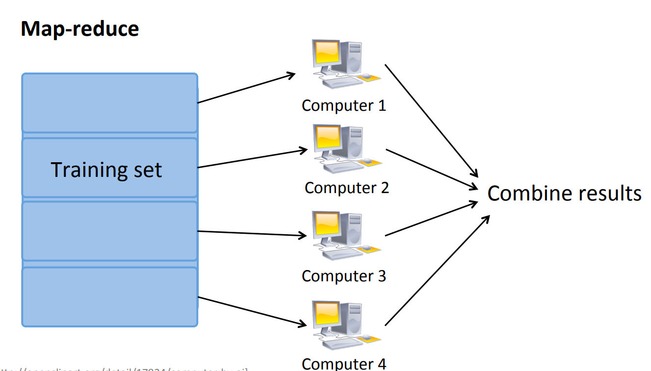
Map-reduce

If the algorithm can be split into parallel parts (e.g. summation), these parts can be assigned to different machines/CPU cores to compute simultaneously to speed up the process.