ML: Support Vector Machine

Source: Coursera Machine Learning provided by Stanford University Andrew Ng - Machine Learning | Coursera

---

Support Vector Machine

hypothesis:

$$ h_{\theta}(x) = \left\{\begin{matrix}0\ \ \ if\ \theta^{T}x < 0 \\1\ \ \ if\ \theta^{T}x \geq 0\end{matrix}\right. $$

cost function:

$$ J(\theta) = C \sum_{i=1}^{m}\left [ y^{(i)} cost_{1}(\theta^{T}x^{(i)}) + (1-y^{(i)})cost_{0}(\theta^{T}x^{(i)})\right ] + \frac{1}{2}\sum_{j=1}^{n}\theta_{j}^{2} $$

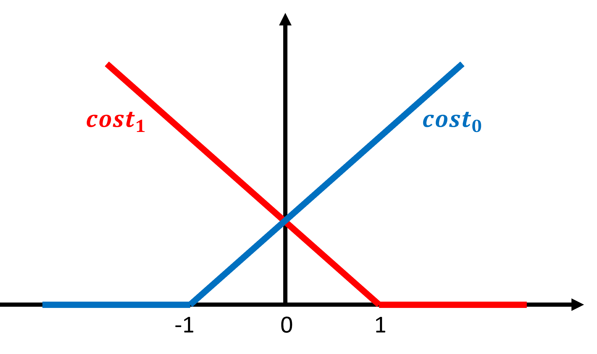
where $C$ is a parameter similar to $\frac{1}{\lambda}$ that controls the penalty for misclassified training examples. A large $C$ will make the SVM try to classify all examples correctly and more prone to overfitting, and vice versa. Note that the term $\frac{1}{m}$ is crossed out, since a constant doesn't affect the result of a minimization problem.

large margin classifier:

SVM is also called a large margin classifier because it finds a decision boundary furthest from the margin of different groups. This is particularly true when $C$ is large. The following is a non-rigorous intuition.

When $C$ is large, SVM tries to classify all examples correctly, making the first term of the cost function $0$. That is:

$$ if\ y^{(i)}=1,\ cost_{1} = 0 \Rightarrow \theta^{T}x^{(i)} = \overrightarrow{\theta} \overrightarrow{x^{(i)}}= p^{(i)}\left\| \theta\right\|\geq 1 $$

$$ if\ y^{(i)}=0,\ cost_{0} = 0 \Rightarrow \theta^{T}x^{(i)} = \overrightarrow{\theta} \overrightarrow{x^{(i)}}= p^{(i)}\left\| \theta\right\|\leq -1 $$

where $p^{(i)}$ is the projection of vector $\overrightarrow{x^{(i)}}$ on vector $\overrightarrow{\theta}$. And the minimization problem becomes:

$$ \underset{\theta}{min} \sum_{j=1}^{n} \theta_{j}^{2} = \left\| \theta \right\|^{2} $$

From the conditions, $\theta$ should satisfy:

$$ \left\| \theta \right\| \geq \frac{1}{\left| p^{(i)}\right|} \Rightarrow \left\| \theta \right\| \geq \frac{1}{\left| p^{(i)}\right|_{min}} $$

To minimize $\left\| \theta \right\|$, whose lowerbound is constrained by $\frac{1}{\left| p^{(i)}\right|_{min}}$, SVM finds a decision boudary with the largest possible $\left| p^{(i)}\right|_{min}$, which is the "margin" (hint: vector $\overrightarrow{\theta}$ is perpendicular to the decision boundary).

kernels:

Kernels are another way to deal with non-linear boundaries. Instead of adding polynomial features, each feature of a training example is replaced by the "similarity" between the original input and a chosen "landmark". Then the trained SVM will classify inputs based on how "close" they are to different landmarks, which are measured by the corresponding $\theta$s.

That is, for each $x^{(i)}$, replace it with $f^{(i)}$:

$$ f^{(i)}=\begin{bmatrix}f_{0}^{(i)} \\f_{1}^{(i)} \\\cdots  \\f_{L}^{(i)}\end{bmatrix} = \begin{bmatrix}1 \\k(x^{(i)},l^{(1)}) \\\cdots \\k(x^{(i)},l^{(L)})\end{bmatrix} $$

where $L$ is the number of landmarks. Generally, the $m$ training examples are chosen as landmarks. That is, $l^{(i)} = x^{(i)}$, $L = m$, and $f^{(i)},\theta \in \mathbb{R}^{m+1}$.

With kernels, the hypothesis and cost function for SVM become:

$$ h_{\theta}(x) = \left\{\begin{matrix}0,\ \ \ if\ \theta^{T}f \geq 0 \\1,\ \ \ if\ \theta^{T}f \leq 0\end{matrix}\right. $$

$$ J(\theta) = C \sum_{i=1}^{m}\left [ y^{(i)} cost_{1}(\theta^{T}f^{(i)}) + (1-y^{(i)})cost_{0}(\theta^{T}f^{(i)})\right ] + \frac{1}{2}\sum_{j=1}^{m}\theta_{j}^{2} $$

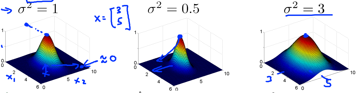
There are different kernel functions for computing "similarity". Not using any function (i.e. not replacing $x$ with $f$) is called "linear kernel". One commonly used kernel is the Gaussian kernel:

$$ k(x,l) = exp(-\frac{\left\| x-l\right\|^2}{2\sigma^2}) $$

This value is 1 when $x$ is the same as $l$ and gradually decreases to 0 as $x$ moves away from $l$. A larger $\sigma^2$ results in a quicker decrease and higher bias, and vice versa:

Note that feature scaling and mean normalization should be performed before using the Gaussian kernel.

Kernels must satisfy Mercer's Theorem to be valid. Other possible kernels include polynomial kernels, String kernel, chi-square kernel, and histogram intersection kernel.

choosing between logistic regression and SVM:

The rough criteria are:

• $n \gg m$: logistic regression or SVM without a kernel (linear kernel), otherwise it's likely to overfit
• $n$ is small, $m$ is intermediate: SVM with Gaussian kernel
• $n \ll m$: add more features, then logistic regression or SVM without a kernel

Neural networks are likely to work well for most of these settings, but may be slower to train.