ML: Logistic Regression | Regularization

Source: Coursera Machine Learning provided by Stanford University Andrew Ng - Machine Learning | Coursera

---

Supervised Learning - Classification / Logistic Regression

terminology:

$y^{(i)}$ is also called the "label" of the i-th training example.

hypothesis: 

$$ h_{\theta}(x) = g(\theta^{T}x) $$

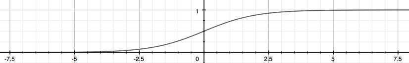
$$ g(z) = \frac{1}{1+e^{-z}} $$

The funcion $g$ is called the sigmoid function looking like: 

In this way, the value of $h_{\theta}(x)$ can be treated as the propabality of the example being positive, i.e.

$$ h_{\theta}(x) = P(y=1|x;\theta) = 1 - P(y=0|x;\theta) $$

decision boundary: 

The classification result can be derived by:

$$ h_{\theta}(x) \geq  0.5 \Rightarrow y=1 $$

$$ h_{\theta}(x) <  0.5 \Rightarrow y=0 $$

According to the property of the sigmoid function, that is:

$$ h_{\theta}(x) = g(\theta^{T}x) \geq 0.5 \Leftrightarrow \theta^{T}x \geq 0 \Rightarrow y=1 $$

$$ h_{\theta}(x) = g(\theta^{T}x) < 0.5 \Leftrightarrow \theta^{T}x < 0 \Rightarrow y=0 $$

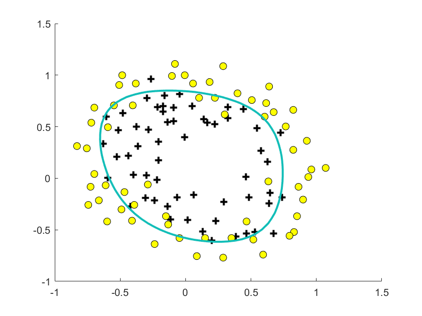
from which the decision boundary can be derived, which is a line separating the area where $y=0$ and $y=1$.

cost function: 

Applying the same cost function as linear regression will result in a non-convex function having many local extrema. The convex cost function for logistic regression is:

$$ J(\theta) = \frac{1}{m} \sum_{i=1}^{m} Cost(h_{\theta}(x^{(i)}),y^{(i)}) $$

$$ Cost(h_{\theta}(x),y) = \left\{\begin{matrix} -log(h_{\theta}(x)), y=1 \\ -log(1-h_{\theta}(x)), y=0 \end{matrix}\right. $$

If $h_{\theta}(x)$ is close to $y$, then the function $Cost$ will output 0, otherwise infinity. For example, if $y=1$ and $h_{\theta}(x) \rightarrow 1$, $Cost \rightarrow 0$, if $y=1$ but $h_{\theta}(x) \rightarrow 0$, $Cost \rightarrow \infty$. The compressed forms are: 

$$ Cost(h_{\theta}(x),y) = -ylog(h_{\theta}(x)) - (1-y)log(1-h_{\theta}(x)) $$

$$ J(\theta) = -\frac{1}{m} \sum_{i=1}^{m} (y^{(i)}log(h_{\theta}(x^{(i)})) + (1-y)log(1-h_{\theta}(x))) $$

multiclass classification - one-vs-all: 

If there are $k$ classes, train k classification models. The k-th model evaluates the probability of the example being in the k-th category:

$$ h_{\theta}^{(k)}(x) = P(y=k|x;\theta) $$

$$ prediction = \underset{i}{max}(h_{\theta}^{(i)}(x)) $$

gradient descent:

The same formula as linear regression, although essentially the hypothesis $h_{\theta}(x)$ is different.

the problem of overfitting: 

	performance	cause
underfitting / high bias	the hypothesis $h_{\theta}$ maps poorly to the trend of the data	the hypothesis being too simple or using too few features
overfitting / high variance	the hypothesis creates many unnecessary curves and angles that it fits the training examples but does not generalize well to predict new data	the hypothesis using too many features

resolutions for overfitting:

• reduce the number of features: manually select which features to keep / use a model selection algorithm

• regularization: keep all the features, but reduce the magnitude of parameters $\theta_{j}$'s, which works well when there are many slightly useful features

regularization: 

By modifying the cost function:

$$ J(\theta) = -\frac{1}{m} \sum_{i=1}^{m} (y^{(i)}log(h_{\theta}(x^{(i)})) + (1-y)log(1-h_{\theta}(x))) + \frac{\lambda}{2m} \sum_{j=1}^{n}\theta_{j}^{2} $$

the magnitude of parameters are taken into account and thus reduced. $\lambda$ is the regularization parameter. If $\lambda$ is too small, the effectiveness of regularization will be too low to address overfitting; if $\lambda$ is too large, underfitting may occur. Note that $\theta_{0} = 1$ is not regularized. 

The gradient descent formula is:

$$ \theta_{0} = \theta_{0} - \frac{\alpha}{m} \sum_{i=1}^{m} (h_{\theta}(x^{(i)})-y^{(i)})x_{0}^{(i)} $$

$$ \theta_{j} = \theta_{j} - \alpha \left [ \left ( \frac{1}{m} \sum_{i=1}^{m} (h_{\theta}(x^{(i)})-y^{(i)})x_{j}^{(i)} \right ) + \frac{\lambda}{m}\theta_{j}\right ] = (1-\frac{\alpha\lambda}{m})\theta_{j} - \frac{\alpha}{m} \sum_{j=1}^{n} (h_{\theta}(x^{(i)})-y^{(i)})x_{j}^{(i)} \ \ \ \ \ j \in [1,n] $$

Because $ 1 - \frac{\alpha\lambda}{m} < 1 $, $\theta_{j}$ can thus be intuitively viewed as reducing by some amount in each iteration. The same process can be applied to linear regression as well.

Regularization is also applicable to normal equation. The modified equation is: 

$$ \theta = (X^{T}X+\lambda L)^{-1}X^{T}y $$

$$ L = \begin{bmatrix}0 &  &  &  \\ & 1 &  &  \\ &  & \ddots &  \\ &  &  & 1 \\\end{bmatrix} $$

where $L$ is a $(n+1)x(n+1)$ matrix. For the initial equation, when $m<n$, $X^{T}X$ is non-invertible; when $m=n$, $X^{T}X$ may be non-invertible. However, when the term $\lambda L$ is added, $X^{T}X+\lambda L$ becomes invertible.

implementation: 

hypothesis:

function g = sigmoid(z)
    g = 1 ./ (1 + exp(-z));
end
h = sigmoid(X * theta);

cost function & gradient (regularized):

function [J, grad] = costFunction(theta, X, y, lambda)
    m = size(y);
    h = sigmoid(X * theta);
    J = - sum(y .* log(h) + (1-y) .* log(1-h)) / m + lambda * sum(theta(2:end) .^ 2) / m;    % don't regularize theta0
    grad = X' * (h - y) / m + lambda / m * theta;
    grad(1) = grad(1) - lambda / m * theta(1);    % don't regularize theta0;
end

advanced optimization: "Conjugate gradient", "BFGS", and "L-BFGS" are more sophisticated, faster ways to optimize $\theta$ that can be used instead of gradient descent. The Matlab built-in function fminuncis one approach.

% set options for fminunc
options = optimoptions(@fminunc,'Algorithm','Quasi-Newton','GradObj', 'on', 'MaxIter', 400);
% initialize the parameters
initial_theta = zeros(size(X,2), 1);
$ run fminunc
[theta, cost] = fminunc(@(t)(costFunction(t, X, y)), initial_theta, options);