Basic knowledge
conditionals
mark= 56
if mark>= 69.5:
    print("distribution")
elif mark>= 59.5:
    print("merit")
elif mark>= 50.0:
    print("pass")
else:
    print("Fail")
pass
Loops
numbers= [1,2,3,4,5,6]
for i in numbers:
    print(i)
1
2
3
4
5
6
number_plus_one= []
number_plus_one= []
for i in numbers:
    number_plus_one.append(i+1)
    print("current number is: "+ str(i))
current number is: 1
current number is: 2
current number is: 3
current number is: 4
current number is: 5
current number is: 6
number_plus_one
[2, 3, 4, 5, 6, 7]
for i in range(1, 8, 2):
    print(i)
1
3
5
7
count= 0
while count< 5:
    print(count)
    count+= 1
0
1
2
3
4
count= 0
while True:
    print(count)
    count+= 1
    if count>= 5:
        break
0
1
2
3
4
Functions
def my_func():
    print("Hello from my func")
my_func()
Hello from my func
def my_func2(greeting, planet):
    print(greeting+ ' '+ planet+ '!')
my_func2('Hello', 'World')
Hello World!
def add(a, b):
    return a+ b
result= add(1, 2)
print(result)
3
result
3
Python packages, and the numpy package
import numpy as np
np.identity(5)
array([[1., 0., 0., 0., 0.],
       [0., 1., 0., 0., 0.],
       [0., 0., 1., 0., 0.],
       [0., 0., 0., 1., 0.],
       [0., 0., 0., 0., 1.]])
from numpy import identity
identity(5)
array([[1., 0., 0., 0., 0.],
       [0., 1., 0., 0., 0.],
       [0., 0., 1., 0., 0.],
       [0., 0., 0., 1., 0.],
       [0., 0., 0., 0., 1.]])
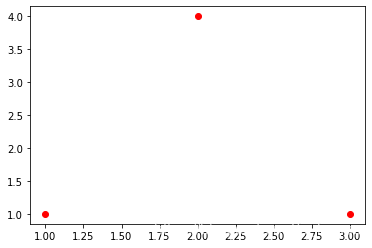
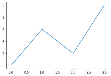
from matplotlib import pyplot as plt
plt.plot([1,2,3],[1,4,1],'or')
[<matplotlib.lines.Line2D at 0x208b1c47780>]
Numpy arrays
import numpy as np
arr= np.array([1.2, 3.14, -6.45])
arr
array([ 1.2 , 3.14, -6.45])
2* [23,42]
[23, 42, 23, 42]
2* arr
array([ 2.4 , 6.28, -12.9 ])
arr+ 1
array([ 2.2 , 4.14, -5.45])
arr* -1
array([-1.2 , -3.14, 6.45])
arr** 2
array([ 1.44 , 9.8596, 41.6025])
arr1= arr
arr2= np.array([1, 2, 3])
print([1, 2 ,3]+ [3, 4, 5]) #list
arr1+ arr2 #numpy array
[1, 2, 3, 3, 4, 5]


array([ 2.2 ,  5.14, -3.45])
arr1* arr2
array([ 1.2 , 6.28, -19.35])
np.sin(1)
0.8414709848078965
np.sin(arr1)
array([ 0.93203909, 0.00159265, -0.16604211])
arr1[0]
1.2
arr[: 2]
array([1.2 , 3.14])
Numpy arrays pt 2
import numpy as np
a= np.array([[1, 2, 3],[4, 5, 6]])
a
array([[1, 2, 3],
       [4, 5, 6]])
a.shape #get the number of rows and cols
(2, 3)
nrows, ncols= a.shape
print(nrows, ncols)
2 3
a.shape= 6
a
array([1, 2, 3, 4, 5, 6])
a.shape= [3, 2]
a
array([[1, 2],
       [3, 4],
       [5, 6]])
a.shape= [2, 3]
a
array([[1, 2, 3],
       [4, 5, 6]])
np.zeros(5)
array([0., 0., 0., 0., 0.])
np.zeros([3, 4])
array([[0., 0., 0., 0.],
       [0., 0., 0., 0.],
       [0., 0., 0., 0.]])
np.ones([3, 4])
array([[1., 1., 1., 1.],
       [1., 1., 1., 1.],
       [1., 1., 1., 1.]])
np.arange(0.1, 0.2, 0.01) #start, stop, step
array([0.1 , 0.11, 0.12, 0.13, 0.14, 0.15, 0.16, 0.17, 0.18, 0.19])
np.linspace(0.1, 0.2, 15) #rather than the step, the third one is the numbers of nums between the start and the stop
array([0.1       , 0.10714286, 0.11428571, 0.12142857, 0.12857143,
       0.13571429, 0.14285714, 0.15      , 0.15714286, 0.16428571,
       0.17142857, 0.17857143, 0.18571429, 0.19285714, 0.2       ])
a= np.array([1, 2, 3])
b= np.array([4, 5, 6])
np.hstack([a, b]) #horizentally
array([1, 2, 3, 4, 5, 6])
np.vstack([a, b]) #vertically
array([[1, 2, 3],
       [4, 5, 6]])
More numpy features (other than arrays)
import numpy as np
np.random.normal(1, 2, 5)# (mean, sd, scale)
array([0.26692905, 3.25555715, 5.55266956, 1.23445221, 1.85074104])
a= np.random.normal(1, 2, 10)
a
array([ 1.61286433, -2.2266842 , -2.06336836,  1.70629078, -0.01086119,
        0.9961519 ,  0.42980328,  4.31010475, -0.07291085, -2.21994622])
np.average(a)
0.2461444230839865
np.var(a)
3.8810147907170185
b= np.random.normal(0, 5, [5, 3])
b
array([[  4.14403725,   4.93392806, -12.57708917],
       [  3.74246174,   1.43706417,  -3.8630664 ],
       [  1.94530969,   6.6532378 ,  -3.39473863],
       [  5.91008478,  -8.03735424,   7.02867261],
       [  4.88898932,   1.91366109,   3.04734046]])
np.average(b)
1.1848359007671332
np.average(b, axis= 0) # axis= 0 :row
array([ 4.12617655, 1.38010737, -1.95177623])
np.average(b, axis= 1) # axis= 1: col
array([-1.16637462, 0.43881984, 1.73460295, 1.63380105, 3.28333029])
m= np.matrix([[1, 2], [4, 5]])
m
matrix([[1, 2],
        [4, 5]])
np.linalg.eig(m) #Compute the eigenvalues and right eigenvectors of a square array
(array([-0.46410162,  6.46410162]), matrix([[-0.80689822, -0.34372377],
         [ 0.59069049, -0.9390708 ]]))
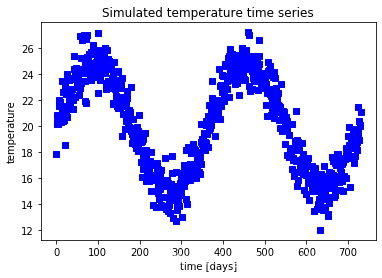
A simple plot with matplotlib
import numpy as np
time = np.linspace(0, 2* 365, 2* 365)
temperature = 20+ 5* np.sin(2* np.pi/ 365* time)
temperature= temperature + np.random.normal(size= 2* 365)
from matplotlib import pyplot as plt
plt.plot(time, temperature, 'sb')
plt.xlabel('time [days]')
plt.ylabel('temperature')
plt.title('Simulated temperature time series')
plt.show()
plt.plot?
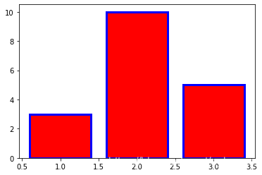
Bar plots
import numpy as np
from matplotlib import pyplot as plt
x= np.array([1,2,3])
y= np.array([3, 10, 5])
plt.bar(x, y, color= 'red', edgecolor= 'blue', linewidth= 3)
plt.show()
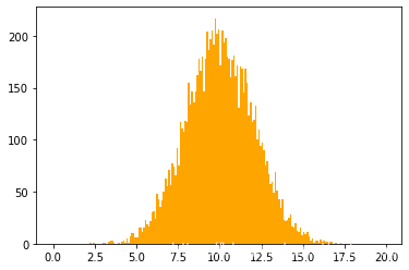
Histograms
import numpy as np
from matplotlib import pyplot as plt
x= np.random.normal(10, 2, size= 10000)
counts, breaks= np.histogram(x, bins= np.arange(0, 20, 0.5))
len(breaks) #40
len(counts) #39
plt.bar(breaks[:-1], counts) #需要去除breaks中的最后一个值
<BarContainer object of 39 artists>
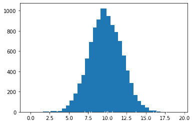
plt.hist(x, bins=np.arange(0, 20, 0.1), color= 'orange')
plt.show()
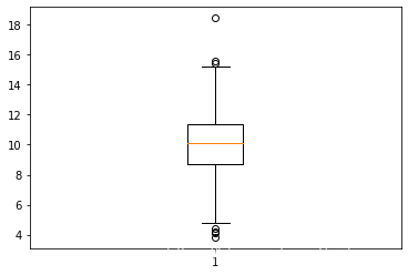
Boxplot
import numpy as np
from matplotlib import pyplot as plt
x= np.random.normal(10, 2, 1000)
plt.boxplot(x)
plt.show()
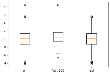
data= [x, x[:100], x[10:]]
plt.boxplot(data, labels= ['all', 'fisrt 100', 'rest'])
plt.show()
Raster plots(光栅图) and contour(等高线) plots
import numpy as np
from matplotlib import pyplot as plt
xx= np.repeat(np.linspace(-2, 2, 50), 50).reshape(50, 50)
yy= np.transpose(xx)
zz= np.exp(-xx**2- yy**2)
plt.matshow(zz, cmap= plt.cm.rainbow)
plt.colorbar()
plt.contour(zz, levels =3, colors= 'black')
plt.show()
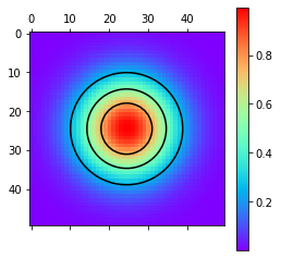
zz.shape
(50, 50)
Geographical maps
from matplotlib import pyplot as plt
from mpl_toolkits.basemap import Basemap
map= Basemap(projection= 'merc', resolution= 'l', llcrnrlat=45, urcrnrlat= 60, llcrnrlon= -10, urcrnrlon= 10)
map.drawcoastlines()
map.drawcountries()
map.fillcontinents(color= 'beige')
map.drawmapboundary(fill_color= 'lightblue')
map.scatter(x= 355, y= 50, latlon= True)
plt.show()

from matplotlib import pyplot as plt
plt.plot([1,4,2,6])
plt.figure(figsize=[6,6])
# plt.savefig('figure1.png')
plt.show()
<Figure size 432x432 with 0 Axes>
Pandas
import pandas as pd
pd? # see the help document
Pandas Series
import pandas as pd
import numpy as np
s= pd.Series([1, 3, 5, np.nan, 6, 8])
s
0    1.0
1    3.0
2    5.0
3    NaN
4    6.0
5    8.0
dtype: float64
s.values
array([ 1., 3., 5., nan, 6., 8.])
s.index
RangeIndex(start=0, stop=6, step=1)
s[4]
6.0
s[: 3]
0    1.0
1    3.0
2    5.0
dtype: float64
s= pd.Series(data= [1, 2, 3], index= ['a', 'b', 'c'])
s
a    1
b    2
c    3
dtype: int64
s[2]
3
s['c']
3
s[0: 2]
a    1
b    2
dtype: int64
s['a':'c']
a    1
b    2
c    3
dtype: int64
population= pd.Series(
    index= ['russia', 'turkey', 'germany', 'france', 'uk'],
    data= [146, 83, 82, 67, 66]
)
population
russia     146
turkey      83
germany     82
france      67
uk          66
dtype: int64
population['uk']
66
Pandas DataFrames
import numpy as np
import pandas as pd
population= pd.Series(
    index= ['russia', 'turkey', 'germany'],
    data= [146, 83, 82]
)
area= pd.Series(
    index= ['russia', 'germany', 'turkey'],
    data= [3995, 357, 783]
)
countries= pd.DataFrame({'population': population, 'area': area})
countries
|
population |
area |
| germany |
82 |
357 |
| russia |
146 |
3995 |
| turkey |
83 |
783 |
Index Series
import pandas as pd
import numpy as np
s= pd.Series(data= [1, 2, 3], index= ['a', 'b', 'c'])
s.index
Index(['a', 'b', 'c'], dtype='object')
s.keys()
Index(['a', 'b', 'c'], dtype='object')
s[1]
2
s['b']
2
s.items()
<zip at 0x209a4e97288>
for index, val in s.items():
    print('index '+ str(index)+ ' '+ ':: value '+ str(val))
index a :: value 1
index b :: value 2
index c :: value 3
s[0: 2]
a    1
b    2
dtype: int64
s['a': 'b']
a    1
b    2
dtype: int64
s[['a', 'c']]
a    1
c    3
dtype: int64
s[s>= 1]
a    1
b    2
c    3
dtype: int64
s[s> 1]
b    2
c    3
dtype: int64
ss= pd.Series(index= [1, 3, 5], data= ['a', 'b', 'c'])
ss
1    a
3    b
5    c
dtype: object
ss[1] #explicit indexing
'a'
ss[0: 3] #implicit indexing
1    a
3    b
5    c
dtype: object
ss.loc[1: 3] #explicit indexing
1    a
3    b
dtype: object
ss.iloc[1]
'b'
Indexing DataFrames
import pandas as pd
import numpy as np
population= pd.Series(
    index= ['russia', 'turkey', 'germany'],
    data= [146, 83, 82]
)
area= pd.Series(
    index= ['russia', 'germany', 'turkey'],
    data= [3995, 357, 783]
)
countries= pd.DataFrame({'population': population, 'area': area})
countries
|
population |
area |
| germany |
82 |
357 |
| russia |
146 |
3995 |
| turkey |
83 |
783 |
countries['area']
germany     357
russia     3995
turkey      783
Name: area, dtype: int64
countries['germany': 'turkey']
|
population |
area |
| germany |
82 |
357 |
| russia |
146 |
3995 |
| turkey |
83 |
783 |
countries['population': 'area']
countries.loc['turkey', :]
population     83
area          783
Name: turkey, dtype: int64
countries.loc['russia']
population     146
area          3995
Name: russia, dtype: int64
countries.loc['russia': 'turkey', 'population']
russia    146
turkey     83
Name: population, dtype: int64
countries.loc[:, 'area']
germany     357
russia     3995
turkey      783
Name: area, dtype: int64
countries.iloc[0, 0]
82
countries.iloc[1] # extract the specific row
population     146
area          3995
Name: russia, dtype: int64
countries.iloc[:, 1] # all rows and area
germany     357
russia     3995
turkey      783
Name: area, dtype: int64
Add/ Removing coloums
import pandas as pd
df= pd.DataFrame({'x':[1,2,3], 'y': ['a', 'b', 'c']})
df
df['z']= [True, False, True]
df
|
x |
y |
x_squared |
z |
| 0 |
1 |
a |
1 |
True |
| 1 |
2 |
b |
4 |
False |
| 2 |
3 |
c |
9 |
True |
df['x_squared']= df['x']** 2
df
|
x |
y |
z |
x_squared |
| 0 |
1 |
a |
True |
1 |
| 1 |
2 |
b |
False |
4 |
| 2 |
3 |
c |
True |
9 |
df.drop('z', axis= 1) # col: axis= 1, row: axis= 0
|
x |
y |
x_squared |
| 0 |
1 |
a |
1 |
| 1 |
2 |
b |
4 |
| 2 |
3 |
c |
9 |
df # but the original data has not been manipulated
|
x |
y |
z |
x_squared |
| 0 |
1 |
a |
True |
1 |
| 1 |
2 |
b |
False |
4 |
| 2 |
3 |
c |
True |
9 |
df= df.drop('z', axis= 1)
df
|
x |
y |
x_squared |
| 0 |
1 |
a |
1 |
| 1 |
2 |
b |
4 |
| 2 |
3 |
c |
9 |
Filtering Rows
import numpy as np
import pandas as pd
df= pd.DataFrame({'x': np.random.normal(size= 10)})
df
|
x |
| 0 |
0.862766 |
| 1 |
-1.622989 |
| 2 |
0.211018 |
| 3 |
1.000474 |
| 4 |
0.568656 |
| 5 |
1.021812 |
| 6 |
0.424689 |
| 7 |
0.273512 |
| 8 |
-0.913785 |
| 9 |
0.599780 |
df.drop(0, axis= 0) # remove the first row, not permanently
|
x |
| 1 |
-1.622989 |
| 2 |
0.211018 |
| 3 |
1.000474 |
| 4 |
0.568656 |
| 5 |
1.021812 |
| 6 |
0.424689 |
| 7 |
0.273512 |
| 8 |
-0.913785 |
| 9 |
0.599780 |
df.drop([1, 2, 3], inplace= True) # remove these rows permanently: set inpalce= True
df
|
x |
| 0 |
0.862766 |
| 4 |
0.568656 |
| 5 |
1.021812 |
| 6 |
0.424689 |
| 7 |
0.273512 |
| 8 |
-0.913785 |
| 9 |
0.599780 |
df[(df['x']> 0) & (df['x']< 1)] # positive values
|
x |
| 0 |
0.862766 |
| 4 |
0.568656 |
| 6 |
0.424689 |
| 7 |
0.273512 |
| 9 |
0.599780 |
df.query('x> 0 & x< 1')
|
x |
| 0 |
0.862766 |
| 4 |
0.568656 |
| 6 |
0.424689 |
| 7 |
0.273512 |
| 9 |
0.599780 |
Combining , merging, joining, DataFrames
import pandas as pd
df1= pd.DataFrame({'x': ['a', 'b']}, index= [1, 2])
df2= pd.DataFrame({'x': ['c', 'd']}, index= [3, 4])
pd.concat([df1, df2])
df3= pd.DataFrame({'x': ['a', 'b']}, index= [1, 2])
df4= pd.DataFrame({'y': ['c', 'd']}, index= [1, 2])
pd.concat([df3, df4], axis= 1) # axis= 0,merge them among the rows; axis= 1,merge them among the cols
df5= pd.DataFrame({'x': ['a', 'b']}, index= [1, 2])
df6= pd.DataFrame({'y': ['c', 'd']}, index= [3, 4])
pd.concat([df3, df4])
D:\Users\Howell.L\Anaconda3\lib\site-packages\ipykernel_launcher.py:3: FutureWarning: Sorting because non-concatenation axis is not aligned. A future version
of pandas will change to not sort by default.

To accept the future behavior, pass 'sort=False'.

To retain the current behavior and silence the warning, pass 'sort=True'.

  This is separate from the ipykernel package so we can avoid doing imports until
|
x |
y |
| 1 |
a |
NaN |
| 2 |
b |
NaN |
| 1 |
NaN |
c |
| 2 |
NaN |
d |
Aggregates and group aggregates
import pandas as pd
import numpy as np
df= pd.DataFrame({'product': ['car', 'car', 'fruit', 'fruit'], 'price': [5000, 20000, 0.5, 1.2]})
df
|
product |
price |
| 0 |
car |
5000.0 |
| 1 |
car |
20000.0 |
| 2 |
fruit |
0.5 |
| 3 |
fruit |
1.2 |
df['product'].value_counts()
fruit    2
car      2
Name: product, dtype: int64
df['price'].agg([np.mean, np.min, np.max])
mean     6250.425
amin        0.500
amax    20000.000
Name: price, dtype: float64
df.groupby('product')['price'].agg([np.mean, np.min, np.max])
|
mean |
amin |
amax |
| product |
|
|
|
| car |
12500.00 |
5000.0 |
20000.0 |
| fruit |
0.85 |
0.5 |
1.2 |
Dates and times
import pandas as pd
dates= pd.to_datetime(['2021-01-01 16:20', '1st of Jan, 2021', 'today'])
dates
DatetimeIndex(['2021-01-01 16:20:00', '2021-01-01 00:00:00',
               '2021-05-16 21:10:11.326783'],
              dtype='datetime64[ns]', freq=None)
dates.strftime('%Y-%m-%d')
Index(['2021-01-01', '2021-01-01', '2021-05-16'], dtype='object')
dates.strftime('%Y-%m-%d %H:%M')
Index(['2021-01-01 16:20', '2021-01-01 00:00', '2021-05-16 21:10'], dtype='object')
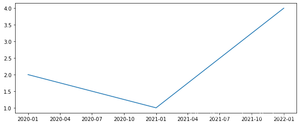
ts= pd.Series(data= [2, 1, 4], index= pd.to_datetime(['2020-01-01', '2021/01/01', '1st Jan 2022']))
ts
2020-01-01    2
2021-01-01    1
2022-01-01    4
dtype: int64
from matplotlib import pyplot as plt
plt.figure(figsize= [10, 4])
plt.plot(ts)
plt.show()
C:\Users\Howell.L\AppData\Roaming\Python\Python37\site-packages\pandas\plotting\_matplotlib\converter.py:103: FutureWarning: Using an implicitly registered datetime converter for a matplotlib plotting method. The converter was registered by pandas on import. Future versions of pandas will require you to explicitly register matplotlib converters.

To register the converters:
	>>> from pandas.plotting import register_matplotlib_converters
	>>> register_matplotlib_converters()
  warnings.warn(msg, FutureWarning)

 浙公网安备 33010602011771号