【数据分析】Kaggle项目之共享单车数据分析(一)
自行车共享系统是一种租赁自行车的方法,注册会员、租车、还车都将通过城市中的站点网络自动完成,通过这个系统人们可以根据需要从一个地方租赁一辆自行车然后骑到自己的目的地归还。
数据提供了跨越两年的每小时租赁数据,包含天气信息和日期信息,训练集由每月前19天的数据组成,测试集是每月第二十天到月底的数据
提出问题
-
通过测试集中的天气等特征值预测会员租赁数量,临时租赁数量和总租赁数量
数据预处理
查看缺失值
    import numpy as np # linear algebra
    import pandas as pd # data processing, CSV file I/O (e.g. pd.read_csv)

    # Input data files are available in the "../input/" directory.
    # For example, running this (by clicking run or pressing Shift+Enter) will list the files in the input directory

    from datetime import datetime
    import warnings
    warnings.filterwarnings('ignore')

    import matplotlib.pyplot as plt
    import seaborn as sns
    sns.set(style='whitegrid',palette='tab10')

    train=pd.read_csv('../input/train.csv')
    train.info()

    test = pd.read_csv('../input/test.csv')
    test.info()
数据没有缺失值,但是没有缺失值不代表没有异常
检查异常值
train.describe()
先从数值型数据入手,看出租赁额(count)数值差异较大,所以希望观察一下count的密度分布
    # 观察租赁额密度分布
    fig = plt.figure()
    ax = fig.add_subplot(1,1,1)
    fig.set_size_inches(6,5)

    sns.distplot(train['count'])
    ax.set(xlabel='count',title='Distribution of count')
 发现数据密度分布的偏斜比较严重,且有一个很长的尾巴,所以希望能把这一列的长尾处理一下,排除掉3个标准差以外的数据
    # 去除3个标准差
    train_WithoutOutliers = train[np.abs(train['count']-train['count'].mean())<=(3*train['count'].std())]
    train_WithoutOutliers.shape
    train_WithoutOutliers['count'].describe()
    fig = plt.figure()
    ax1 = fig.add_subplot(1,2,1)
    ax2 = fig.add_subplot(1,2,2)
    fig.set_size_inches(12,5)

    sns.distplot(train_WithoutOutliers['count'],ax=ax1)
    sns.distplot(train['count'],ax=ax2)
    ax1.set(xlabel='count',title='Distribution of count without outliers')
    ax2.set(xlabel='registered',title='Distribution of count')
 长尾去掉以后,可以看到数据波动依然很大,而我们希望波动相对稳定,否则容易产生过拟合,选择对数变化,使得数据相对稳定。
    # 对数变换
    yLabels = train_WithoutOutliers['count']
    yLabels_log = np.log(yLabels)
    sns.distplot(yLabels_log)
 对其余的数值型数据进行处理,由于其他数据同时包含在两个数据集中,为方便数据处理,先将两个数据集合并
    # 合并数据集
    Bike_data = pd.concat([train_WithoutOutliers,test],ignore_index=True)
    # Bike_data.shape
    Bike_data.head()
最终需要使用随机森林预测,为了方便查看可视化数据,先把datetime拆分成日期、时段、年份、月份、星期
    from datetime import date
    Bike_data['date'] = Bike_data.datetime.apply(lambda c : c.split( )[0])
    Bike_data['hour'] = Bike_data.datetime.apply(lambda c : c.split( )[1].split(':')[0]).astype('int')
    Bike_data['year'] = Bike_data.datetime.apply(lambda c : c.split( )[0].split('-')[0]).astype('int')
    Bike_data['month'] = Bike_data.datetime.apply(lambda c : c.split( )[0].split('-')[1]).astype('int')
    Bike_data['weekday'] = Bike_data.date.apply(lambda c : datetime.strptime(c,'%Y-%m-%d').isoweekday())
    Bike_data.head()
查看温度,体感温度,湿度,风速这四列数值型数据的分布
    fig,axes = plt.subplots(2,2)
    fig.set_size_inches(12,10)

    sns.distplot(Bike_data['temp'],ax=axes[0,0])
    sns.distplot(Bike_data['atemp'],ax=axes[0,1])
    sns.distplot(Bike_data['humidity'],ax=axes[1,0])
    sns.distplot(Bike_data['windspeed'],ax=axes[1,1])

    axes[0,0].set(xlabel='temp',title='Distribution of temp')
    axes[0,1].set(xlabel='atemp',title='Distribution of atemp')
    axes[1,0].set(xlabel='humidity',title='Distribution of humidity')
    axes[1,1].set(xlabel='windspeed',title='Distribution of windspeed')
 通过这个分布可以发现一些问题,风速的0数据很多,观察发现空缺值在1-6之间,从这里可以推测出来,数据本身是有缺失值的,但是用0来填充了,但这些风速为0的数据会对预测产生干扰,希望使用随机森林根据相同年份,月份,季节,温度,湿度等几个特征来预测一下风速的缺失值
    from sklearn.ensemble import RandomForestRegressor

    Bike_data["windspeed_rfr"]=Bike_data["windspeed"]
    # 将数据分成风速等于0和不等于两部分
    dataWind0 = Bike_data[Bike_data["windspeed_rfr"]==0]
    dataWindNot0 = Bike_data[Bike_data["windspeed_rfr"]!=0]
    #选定模型
    rfModel_wind = RandomForestRegressor(n_estimators=1000,random_state=42)
    # 选定特征值
    windColumns = ["season","weather","humidity","month","temp","year","atemp"]
    # 将风速不等于0的数据作为训练集,fit到RandomForestRegressor之中
    rfModel_wind.fit(dataWindNot0[windColumns], dataWindNot0["windspeed_rfr"])
    #通过训练好的模型预测风速
    wind0Values = rfModel_wind.predict(X= dataWind0[windColumns])
    #将预测的风速填充到风速为零的数据中
    dataWind0.loc[:,"windspeed_rfr"] = wind0Values
    #连接两部分数据
    Bike_data = dataWindNot0.append(dataWind0)
    Bike_data.reset_index(inplace=True)
    Bike_data.drop('index',inplace=True,axis=1)
填充好了以后再画图观察一下这四个特征值的密度分布 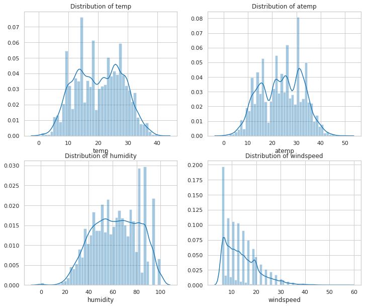
分析数据
可视化并观察数据
整体观察 问题是希望预测每小时总的租赁额,首先整体看一下租赁额相关的三个值和其他特征值的关系
    sns.pairplot(Bike_data,x_vars=['holiday','workingday','weather','season','weekday','hour','windspeed_rfr','humidity','temp','atemp'],
                y_vars=['casual','registered','count'],plot_kws={'alpha':0.1})
 可以得到如下结论:
-
会员在工作日出行多,节假日出行少,临时用户则相反
-
第一季度出行人数总体偏少
-
租赁数量随着天气等级的上升而减少
-
小时数对租赁情况影响明显,会员呈现两个高峰,非会员呈现一个正态分布
-
租赁数量随风速增大而减少
-
温度、湿度对非会员影响比较大,对会员影响较小
下面查看各个特征与每小时租车总量(count)的相关性,由上图可以看出特征值与租车数量基本是线性相关,所以求他们的相关系数
    # 相关性矩阵
    corrDf = Bike_data.corr()

    # ascending = False表示按降序排列
    corrDf['count'].sort_values(ascending = False)
 可以看出特征值对租赁数量的影响力度为,时段>温度>湿度>年份>月份>季节>天气等级>风速>星期几>是否工作日>是否节假日,接下来再看一下共享单车的整体使用情况。

 浙公网安备 33010602011771号