[CV] 计算机视觉像素位变换（反转变换、对数变换，伽马变换，直方图均衡化）

使用工具

opencv 4.7.1
python 3.8

辅助函数

绘制灰度直方图

def drawGrayHistogram(mat, figure: int = 1, title: str = "灰度直方图"):
    '''
        绘制灰度直方图
    '''
    plt.figure(figure)
    plt.hist(mat.flatten(), bins=100, facecolor="#2c3e50",
             edgecolor="#fff", alpha=0.7, density=True, stacked=True)
    plt.xlabel("灰度")
    plt.ylabel("频率")
    plt.title(title)
    plt.savefig(resourcePath+title)

绘制函数变换图

def drawTransformFunction(x, y, figure=1, title="", label=""):
    '''
        绘制转换函数
    '''
    plt.figure(figure)
    plt.title(title)
    plt.plot(x, y,  label=label)
    plt.legend()
    plt.savefig(resourcePath+title)

常见的像素变换算法

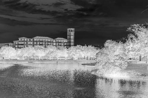
反转变换：即转换后的灰度值=灰度级-像素灰度值

reverseGray = 255-grayMat
cv2.imshow("reverseGray",reverseGray)

原灰度图

转换后的灰度图

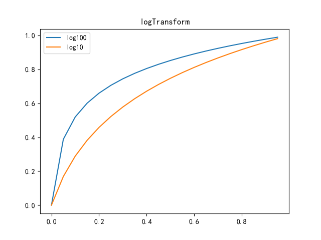
对数变换:公式对应 \(c*log_(v+1)(1.0+v*r)\) 其中r的范围[0,1]

def logTransform(mat, v: float = 1.0, c: float = 1.0):
    '''
        对数变换，v为底数
    '''
    x = np.arange(0, 1, 0.05)
    y = c * np.log(1.0+v*x)/np.log(v+1)
    drawTransformFunction(x, y, 5, "logTransform", "log{}".format(v))
    cvt2mat = mat.astype(np.float64)/255  # 归一化像素
    cvt2mat = c * np.log(1.0+v*cvt2mat)/np.log(v+1)*255  # 对数变换，还原为0~255
    cvt2mat = cvt2mat.astype(np.uint8)  
    return cvt2mat

转换的函数图

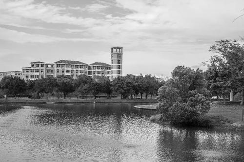
对比：
转换前:

转换后v取10：

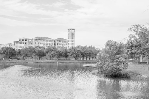
v取100：

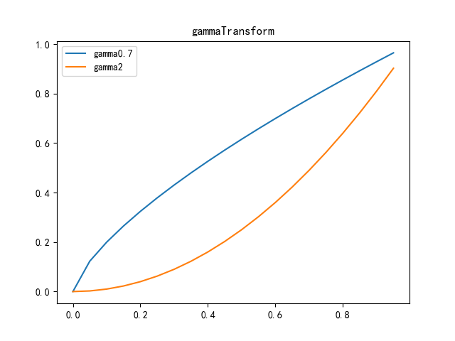
幂律变换（伽马变换）
公式 \(y=c*x^\gamma\)

def gammaTransform(mat, gamma: float = 1.0, c: float = 1.0):
    '''
        幂律变换（伽马变换），gamma为指数
    '''
    x = np.arange(0, 1, 0.05)  # 绘制函数曲线
    y = c * np.power(x, gamma)
    drawTransformFunction(x, y, 4, "gammaTransform", "gamma{}".format(gamma))
    cvt2mat = mat.astype(np.float64)/255  # 归一化
    cvt2mat = c * np.power(cvt2mat, gamma)*255
    cvt2mat = cvt2mat.astype(np.uint8)
    return cvt2mat

变换函数：

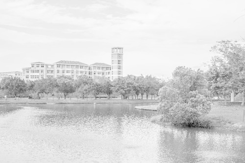
变换前:

Gamma2:

Gamma0.7:

灰度直方图：指的是[0,L-1] (L指的是灰度等级，在opencv中默认为256)
获取灰度值出现的频率并绘制直方图

def drawGrayHistogram(mat, figure: int = 1, title: str = "灰度直方图"):
    '''
        绘制灰度直方图
    '''
    plt.figure(figure)
    plt.hist(mat.flatten(), bins=100, facecolor="#2c3e50",
             edgecolor="#fff", alpha=0.7, density=True, stacked=True)
    plt.xlabel("灰度")
    plt.ylabel("频率")
    plt.title(title)
    plt.savefig(resourcePath+title)

通过定义可以构造一个获取长度为L的一维数组，对灰度值进行计数

def getGrayHistogram(mat, level: int = 256):
    '''
        获取一维灰度为level级别的直方图
    '''
    grayArray = np.zeros(level, dtype=np.uint32)
    for pixel in np.nditer(mat):
        grayArray[pixel] = grayArray[pixel]+1
    return grayArray

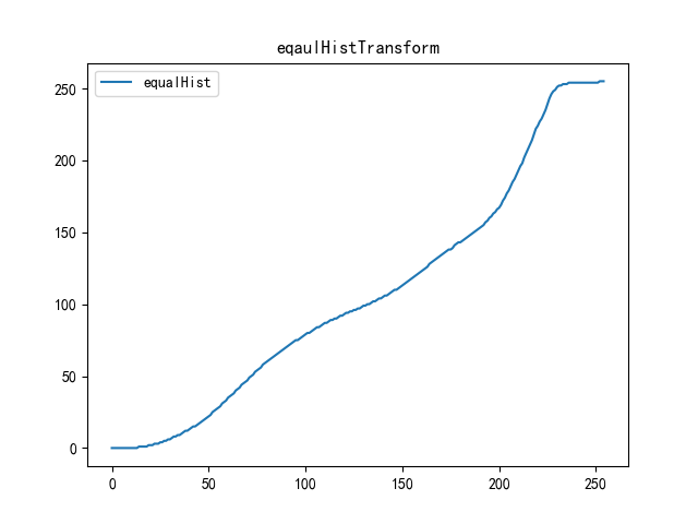
通过灰度值统计数组，使用对应的公式获取离散变换函数\(f(x)=(L-1)/(pixelsCount)*\sum_0^x(h[x])\)，并直接对原矩阵进行映射返回映射后的值

def equalHistTransform(mat, histogram, level: int = 256):
    '''
        均衡化直方图变换
    '''
    csum = np.cumsum(histogram)
    a = (level-1)/csum[level-1]
    mapper = (a*csum).astype(np.uint8)
    x = np.arange(0, 255, 1)
    y = mapper[x]
    drawTransformFunction(x, y, 3, "equalHistTransform", "equalHist")
    return mapper[mat]

变换曲线：

变换前：


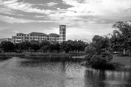
均衡后：