networkx整理
1、基础知识
1.1、介绍
networkx在2002年5月产生,是一个用Python语言开发的图论与复杂网络建模工具,内置了常用的图与复杂网络分析算法,可以方便的进行复杂网络数据分析、仿真建模等工作。
networkx支持创建简单无向图、有向图和多重图;内置许多标准的图论算法,节点可为任意数据;支持任意的边值维度,功能丰富,简单易用。
1.2、作用
利用networkx可以以标准化和非标准化的数据格式存储网络、生成多种随机网络和经典网络、分析网络结构、建立网络模型、设计新的网络算法、进行网络绘制等。
1.3、Graph
1.3.1、Graph的定义
Graph是用点和线来刻画离散事物集合中的每对事物间以某种方式相联系的数学模型。
网络作为图的一个重要领域,包含的概念与定义更多,如有向图网络(Directed Graphs and Networks)、无向图网络(Undirected)等概念。
Graph在现实世界中随处可见,如交通运输图、旅游图、流程图等。此处我们只考虑由点和线所组成的图。
利用图可以描述现实生活中的许多事物,如用点可以表示交叉口,点之间的连线表示路径,这样就可以轻而易举的描绘出一个交通运输网络。
1.3.2、Graph的结构
根据Graph的定义,一个Graph包含一个节点集合和一个边集。
在NetworkX中,一个节点可以是任意hash对象(除了None对象),一条边也可以关联任意的对象,像一个文本字符串,一幅图像,一个XML对象,甚至是另一个图或任意定制的节点对象。
注意:Python中的None对象是不可以作为节点的类型的。
节点与边能够存储任意类型字典的属性和任意其他丰富类型的数据。
1.3.3、Graph分类
- Graph:指无向图(undirected Graph),即忽略了两节点间边的方向。
- DiGraph:指有向图(directed Graph),即考虑了边的有向性。
- MultiGraph:指多重无向图,即两个结点之间的边数多于一条,又允许顶点通过同一条边和自己关联。
- MultiDiGraph:多重图的有向版本。
G = nx.Graph() # 创建无向图

G = nx.DiGraph() # 创建有向图

G = nx.MultiGraph() # 创建多重无向图

G = nx.MultiDigraph() # 创建多重有向图

G.clear() #清空图
2、基本操作
2.1、无向图
- 节点
————如果添加的节点和边是已经存在的,是不会报错的,NetworkX会自动忽略掉已经存在的边和节点的添加。
#添加节点
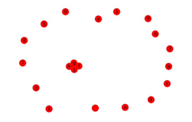
import networkx as nx import matplotlib.pyplot as plt G = nx.Graph() #建立一个空的无向图G G.add_node('a') #添加一个节点1 G.add_nodes_from(['b','c','d','e']) #加点集合 G.add_cycle(['f','g','h','j']) #加环 H = nx.path_graph(10) #返回由10个节点挨个连接的无向图,所以有9条边 G.add_nodes_from(H) #创建一个子图H加入G G.add_node(H) #直接将图作为节点 nx.draw(G, with_labels=True) plt.show()
#访问节点

print('图中所有的节点', G.nodes())

print('图中节点的个数', G.number_of_nodes())
![]()
#删除节点

G.remove_node(1)    #删除指定节点
G.remove_nodes_from(['b','c','d','e'])    #删除集合中的节点

nx.draw(G, with_labels=True)

plt.show()

- 边
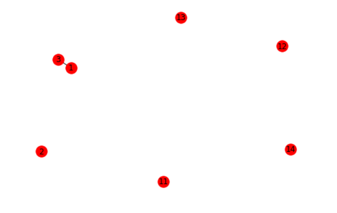
#添加边

F = nx.Graph() # 创建无向图
F.add_edge(11,12)   #一次添加一条边

#等价于
e=(13,14)        #e是一个元组
F.add_edge(*e) #这是python中解包裹的过程

F.add_edges_from([(1,2),(1,3)])     #通过添加list来添加多条边

#通过添加任何ebunch来添加边
F.add_edges_from(H.edges()) #不能写作F.add_edges_from(H)

nx.draw(F, with_labels=True)
plt.show()
#访问边

print('图中所有的边', F.edges())

print('图中边的个数', F.number_of_edges())

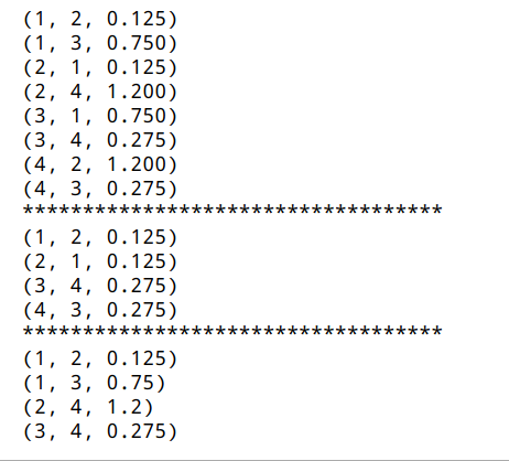
#快速遍历每一条边,可以使用邻接迭代器实现,对于无向图,每一条边相当于两条有向边
FG = nx.Graph()
FG.add_weighted_edges_from([(1,2,0.125), (1,3,0.75), (2,4,1.2), (3,4,0.275)])
for n, nbrs in FG.adjacency():
    for nbr, eattr in nbrs.items():
        data = eattr['weight']
        print('(%d, %d, %0.3f)' % (n,nbr,data))

print('***********************************')

#筛选weight小于0.5的边:
FG = nx.Graph()
FG.add_weighted_edges_from([(1,2,0.125), (1,3,0.75), (2,4,1.2), (3,4,0.275)])
for n, nbrs in FG.adjacency():
    for nbr, eattr in nbrs.items():
        data = eattr['weight']
        if data < 0.5:
            print('(%d, %d, %0.3f)' % (n,nbr,data))
print('***********************************')

#一种方便的访问所有边的方法:
for u,v,d in FG.edges(data = 'weight'):
    print((u,v,d))
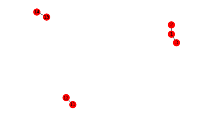
#删除边

F.remove_edge(1,2)
F.remove_edges_from([(11,12), (13,14)])

nx.draw(F, with_labels=True)

plt.show()
- 属性
属性诸如weight,labels,colors,或者任何对象,你都可以附加到图、节点或边上。
对于每一个图、节点和边都可以在关联的属性字典中保存一个(多个)键-值对。
默认情况下这些是一个空的字典,但是我们可以增加或者是改变这些属性。
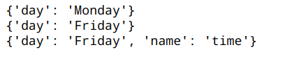
#图的属性

import networkx as nx
import matplotlib.pyplot as plt

G = nx.Graph(day='Monday')    #可以在创建图时分配图的属性
print(G.graph)

G.graph['day'] = 'Friday'     #也可以修改已有的属性
print(G.graph)

G.graph['name'] = 'time'      #可以随时添加新的属性到图中
print(G.graph)
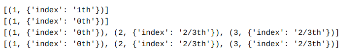
#节点的属性

G = nx.Graph(day='Monday')
G.add_node(1, index='1th')             #在添加节点时分配节点属性
print(G.node(data=True))

G.node[1]['index'] = '0th'             #通过G.node[][]来添加或修改属性
print(G.node(data=True))

G.add_nodes_from([2,3], index='2/3th') #从集合中添加节点时分配属性
print(G.nodes(data=True))

print(G.node(data=True))
#边的属性

G = nx.Graph(day='manday')
G.add_edge(1,2,weight=10)                    #在添加边时分配属性
print(G.edges(data=True))

G.add_edges_from([(1,3), (4,5)], len=22)     #从集合中添加边时分配属性
print(G.edges(data='len'))

G.add_edges_from([(3,4,{'hight':10}),(1,4,{'high':'unknow'})])
print(G.edges(data=True))

G[1][2]['weight'] = 100000                   #通过G[][][]来添加或修改属性
print(G.edges(data=True))

注意:
注意什么时候使用‘=’,什么时候使用‘:’;什么时候有引号什么时候没有引号。
特殊属性weight应该是一个数值型的,并且在算法需要使用weight时保存该数值。
2.2、其他图
有向图和多重图的基本操作与无向图一致。
无向图与有向图之间可以相互转换,转化方法如下:
#有向图转化成无向图

H=DG.to_undirected()
#或者
H=nx.Graph(DG)

#无向图转化成有向图

F = H.to_directed()
#或者
F = nx.DiGraph(H)
3、Functions
-
图
degree(G[, nbunch, weight]):返回单个节点或nbunch节点的度数视图。
degree_histogram(G):返回每个度值的频率列表。
density(G):返回图的密度。
info(G[, n]):打印图G或节点n的简短信息摘要。
create_empty_copy(G[, with_data]):返回图G删除所有的边的拷贝。
is_directed(G):如果图是有向的,返回true。
add_star(G_to_add_to, nodes_for_star, **attr):在图形G_to_add_to上添加一个星形。
add_path(G_to_add_to, nodes_for_path, **attr):在图G_to_add_to中添加一条路径。
add_cycle(G_to_add_to, nodes_for_cycle, **attr):向图形G_to_add_to添加一个循环。
-
节点
nodes(G):在图节点上返回一个迭代器。
number_of_nodes(G):返回图中节点的数量。
all_neighbors(graph, node):返回图中节点的所有邻居。
non_neighbors(graph, node):返回图中没有邻居的节点。
common_neighbors(G, u, v):返回图中两个节点的公共邻居。
-
边
edges(G[, nbunch]):返回与nbunch中的节点相关的边的视图。
number_of_edges(G):返回图中边的数目。
non_edges(graph):返回图中不存在的边。
-
实例:在networkx中列出特定的节点或边缘
import networkx as nx
import matplotlib.pyplot as plt
G = nx.DiGraph()
G.add_edges_from([('n', 'n1'), ('n', 'n2'), ('n', 'n3')])
G.add_edges_from([('n4', 'n41'), ('n1', 'n11'), ('n1', 'n12'), ('n1', 'n13')])
G.add_edges_from([('n2', 'n21'), ('n2', 'n22')])
G.add_edges_from([('n13', 'n131'), ('n22', 'n221')])
G.add_edges_from([('n131', 'n221'), ('n221', 'n131')])
G.add_node('n5')
nx.draw(G, with_labels=True)
plt.show()

1、使用out_degree函数查找所有带有子项的节点:
>>> [k for k,v in G.out_degree().iteritems() if v > 0]
['n13', 'n', 'n131', 'n1', 'n22', 'n2', 'n221', 'n4']
2、所有没有孩子的节点:
>>> [k for k,v in G.out_degree().iteritems() if v == 0]
['n12', 'n11', 'n3', 'n41', 'n21', 'n5']
3、所有孤儿节点,即度数为0的节点:
>>> [k for k,v in G.degree().iteritems() if v == 0]
['n5']
4、超过2个孩子的节点:
>>> [k for k,v in G.out_degree().iteritems() if v > 2]
['n', 'n1']
4、经典图论算法
-
最短路径
函数调用:
dijkstra_path(G, source, target, weight='weight') ————求最短路径
dijkstra_path_length(G, source, target, weight='weight') ————求最短距离
示例:
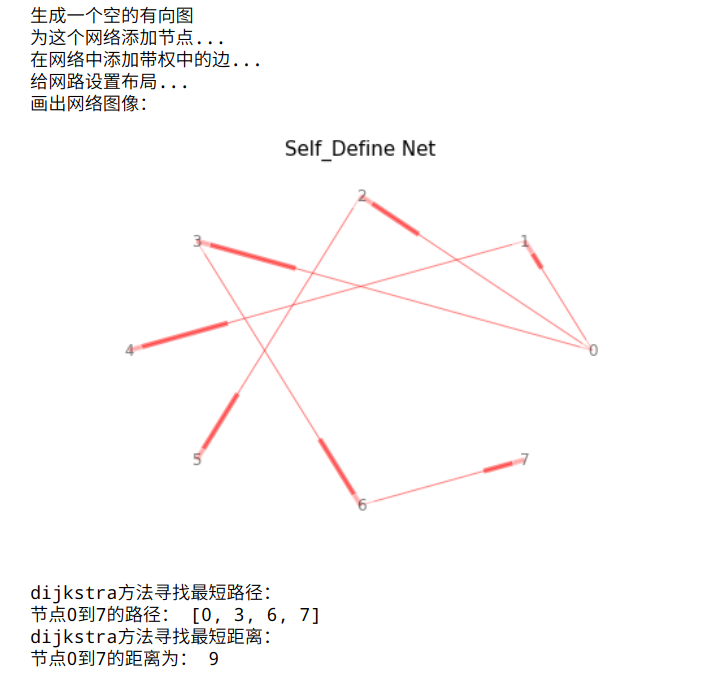
import networkx as nx
import pylab
import numpy as np
#自定义网络
row=np.array([0,0,0,1,2,3,6])
col=np.array([1,2,3,4,5,6,7])
value=np.array([1,2,1,8,1,3,5])

print('生成一个空的有向图')
G=nx.DiGraph()
print('为这个网络添加节点...')
for i in range(0,np.size(col)+1):
    G.add_node(i)
print('在网络中添加带权中的边...')
for i in range(np.size(row)):
    G.add_weighted_edges_from([(row[i],col[i],value[i])])

print('给网路设置布局...')
pos=nx.shell_layout(G)
print('画出网络图像:')
nx.draw(G,pos,with_labels=True, node_color='white', edge_color='red', node_size=400, alpha=0.5 )
pylab.title('Self_Define Net',fontsize=15)
pylab.show()


'''
Shortest Path with dijkstra_path
'''
print('dijkstra方法寻找最短路径:')
path=nx.dijkstra_path(G, source=0, target=7)
print('节点0到7的路径:', path)
print('dijkstra方法寻找最短距离:')
distance=nx.dijkstra_path_length(G, source=0, target=7)
print('节点0到7的距离为:', distance)
-
最小生成树
定义:一个有 n 个结点的连通图的生成树是原图的极小连通子图,且包含原图中的所有 n 个结点,并且有保持图连通的最少的边。
示例:
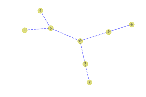
def prim(G, s):
    dist = {}   # dist记录到节点的最小距离
    parent = {} # parent记录最小生成树的双亲表
    Q = list(G.nodes()) # Q包含所有未被生成树覆盖的节点
    MAXDIST = 9999.99    # MAXDIST表示正无穷,即两节点不邻接

    # 初始化数据
    # 所有节点的最小距离设为MAXDIST,父节点设为None
    for v in G.nodes():
        dist[v] = MAXDIST
        parent[v] = None
    # 到开始节点s的距离设为0
    dist[s] = 0

    # 不断从Q中取出“最近”的节点加入最小生成树
    # 当Q为空时停止循环,算法结束
    while Q:
        # 取出“最近”的节点u,把u加入最小生成树
        u = Q[0]
        for v in Q:
            if (dist[v] < dist[u]):
                u = v
        Q.remove(u)

        # 更新u的邻接节点的最小距离
        for v in G.adj[u]:
            if (v in Q) and (G[u][v]['weight'] < dist[v]):
                parent[v] = u
                dist[v] = G[u][v]['weight']
    # 算法结束,以双亲表的形式返回最小生成树
    return parent
import matplotlib.pyplot as plt
import networkx as nx

g_data = [(1, 2, 1.3), (1, 3, 2.1), (1, 4, 0.9), (1, 5, 0.7), (1, 6, 1.8), (1, 7, 2.0), (1, 8, 1.8), (2, 3, 0.9), (2, 4, 1.8), (2, 5, 1.2), (2, 6, 2.8), (2, 7, 2.3), (2, 8, 1.1), (3, 4, 2.6), (3, 5, 1.7), (3, 6, 2.5), (3, 7, 1.9), (3, 8, 1.0), (4, 5, 0.7), (4, 6, 1.6), (4, 7, 1.5), (4, 8, 0.9), (5, 6, 0.9), (5, 7, 1.1), (5, 8, 0.8), (6, 7, 0.6), (6, 8, 1.0), (7, 8, 0.5)]

def draw(g):
    pos = nx.spring_layout(g)
    nx.draw(g, pos, \
            arrows=True, \
            with_labels=True, \
            nodelist=g.nodes(), \
            style='dashed', \
            edge_color='b', \
            width=2, \
            node_color='y', \
            alpha=0.5)
    plt.show()

g = nx.Graph()
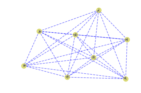
tree = prim(g, 1)

mtg = nx.Graph()
mtg.add_edges_from(tree.items())
mtg.remove_node(None)

draw(mtg)
-
最大联通子图及联通子图规模排序
import matplotlib.pyplot as plt
import networkx as nx
G=nx.path_graph(4)
G.add_path([10,11,12])
nx.draw(G,with_labels=True,label_size=1000,node_size=1000,font_size=20)
plt.show()
#[print(len(c)) for c in sorted(nx.connected_components(G),key=len,reverse=True)]
for c in sorted(nx.connected_components(G),key=len,reverse=True):
    print(c)      #看看返回来的是什么?结果是{0,1,2,3}
    print(type(c))   #类型是set
    print(len(c))   #长度分别是4和3(因为reverse=True,降序排列)


largest_components=max(nx.connected_components(G),key=len)  # 高效找出最大的联通成分,其实就是sorted里面的No.1
print(largest_components)  #找出最大联通成分,返回是一个set{0,1,2,3}
print(len(largest_components))  #4
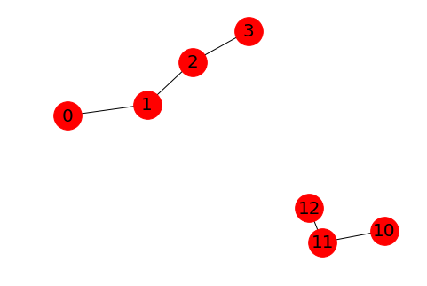
{0, 1, 2, 3}
<class 'set'>
4
{10, 11, 12}
<class 'set'>
3
{0, 1, 2, 3}
4
参考资料:
http://yoghurt-lee.online/2017/03/30/graph-visible/
http://blog.sciencenet.cn/home.php?mod=space&uid=404069&do=blog&id=337442
http://www.cnblogs.com/kaituorensheng/p/5423131.html#_label3
http://baiyejianxin.iteye.com/blog/1764048
https://zhuanlan.zhihu.com/p/33616557
https://blog.csdn.net/qq_31192383/article/details/53748129
https://blog.csdn.net/newbieMath/article/details/73800374
http://osask.cn/front/ask/view/565531

 浙公网安备 33010602011771号