python课程设计-网络欺凌数据检测

一、选题背景

随着社交媒体在每个年龄段的使用越来越普遍，绝大多数公民都依赖于这一基本媒体进行日常沟通。社交媒体的无处不在意味着网络欺凌可以在任何时间、任何地点有效地影响任何人，而互联网的相对匿名性使得此类人身攻击比传统欺凌更难以阻止。所以本次课程设计基于机器学习的网络欺凌检测，特别关注识别网络欺凌者攻击的受害者的特定属性：年龄、种族、性别、宗教或其他网络欺凌。通过检测恶意推文，从而在其发展到网络欺凌水平之前阻止伤害。

二、大数据分析设计方案

1.在课程实践中，所得到的数据会存在有缺失值、重复值等，使用之前需要进行数据预处理。数据预处理没有标准的流程，通常针对不同的任务和数据集属性的不同而不同。对采用数据集先进行去除唯一属性、处理缺失值、表情符号处理、等预处理，通过对各类网络欺凌进行了类型统计、并进行了相关的可视化工作，在原始数据中筛选出更好的数据特征，以提升模型的训练效果。

2.在做完数据预处理和特征提取之后需进一步利用算法来进行结果预测，使用LOGISTIC回归、支持向量机、神经网络、随机森林、朴素贝叶斯等分类技术来进行本次的算法模型。通过算法模型精准度的对比从而能更好的在社交媒体上进行网络欺凌识别。

三、数据分析步骤

1.数据源

采用公开数据集：https://www.kaggle.com/datasets/andrewmvd/cyberbullying-classification

2.数据清洗

对所需的库进行导入：

import numpy as np
import pandas as pd
import matplotlib.pyplot as plt
import seaborn as sns
import plotly.express as px

df = pd.read_csv('/Users/xzh/cyberbullying_tweets.csv')  # 导入数据

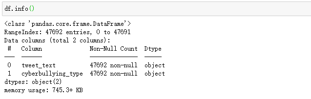
在工程实践中，所得到的数据会存在有缺失值、重复值等，在使用之前需要进行数据预处理。对文本进行特征提取之前，需要将这部分先进行剔除处理：

import warnings
warnings.filterwarnings("ignore")
from warnings import simplefilter
from sklearn.exceptions import ConvergenceWarning
simplefilter("ignore", category=ConvergenceWarning)

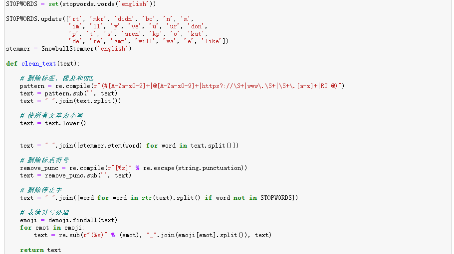
将清理函数应用于文本数据：

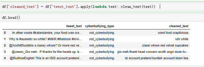
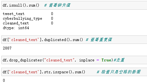
在经过上述的文本处理后得到一分都是小写且不含表情以及第三方链接及停止词的文本数据，在此基础上对文本进一步进行缺失值、重复值处理:

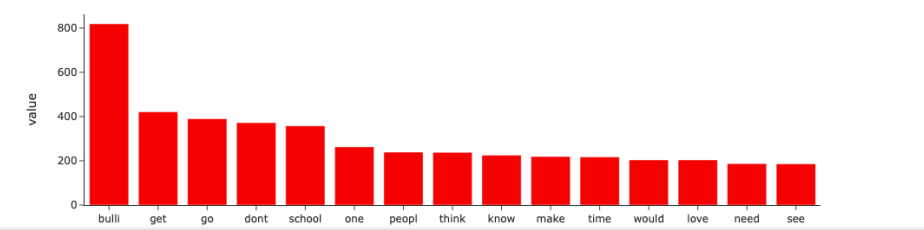
其次对各类网络欺凌进行了类型统计、并进行了相关的可视化工作、并查看了每种欺凌类型的前15的单词分布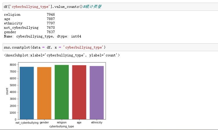

从上图中可得知本次的文本数据的各类网络欺凌类型分布较为均匀。

  绘制每种网络欺凌类型的前15个单词：

for cyber_type in df.cyberbullying_type.unique():
    top50_word = df.cleaned_text[df.cyberbullying_type==cyber_type].str.split(expand=True).stack().value_counts()[:15]
    fig = px.bar(top50_word, color=top50_word.values, color_continuous_scale=px.colors.sequential.RdPu, custom_data=[top50_word.values])
    fig.update_traces(marker_color='red')
    fig.update_traces(hovertemplate='<b>Count: </b>%{customdata[0]}')
    fig.update_layout(title=f"Top 15 words for {cyber_type}",
                     template='simple_white',
                     hovermode='x unified')
    fig.show()

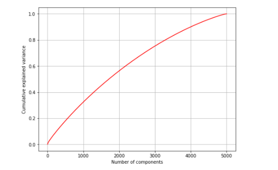
通过网上查找资料本次课程使用到特征提取，通过TF-IDF算法提取了前5000个重要特征，并对其采用了PCA的方法来进行降纬

#从文本数据中使用TF-IDF矢量器提取前5000个最重要的特征
tfidf = TfidfVectorizer(max_features = 5000)  # 使用主成分分析进行降维
from sklearn.decomposition import PCA
NUM_COMPONENTS = 5000  # 特征总数
pca = PCA(NUM_COMPONENTS)
reduced = pca.fit(scaled_X_train)

得到数据关系如图：

3.数据分析采用算法

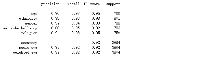
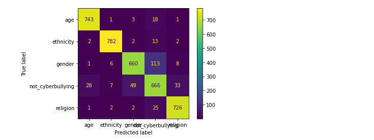
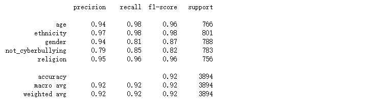
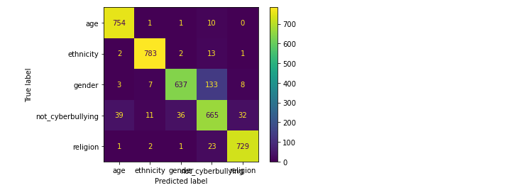
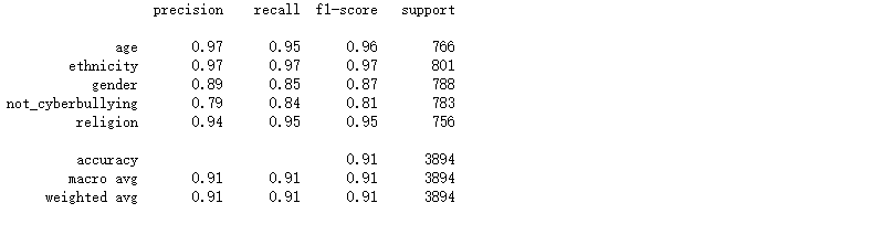
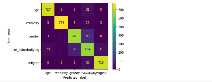
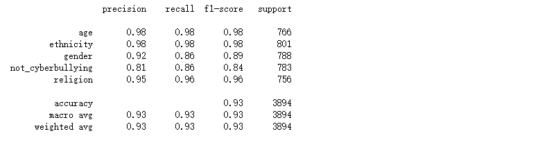
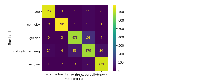
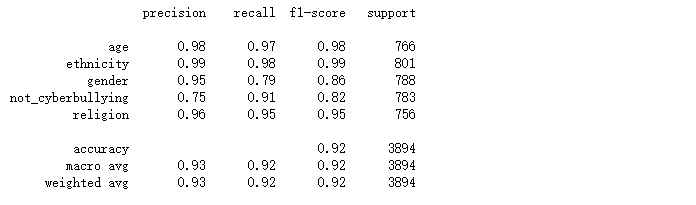
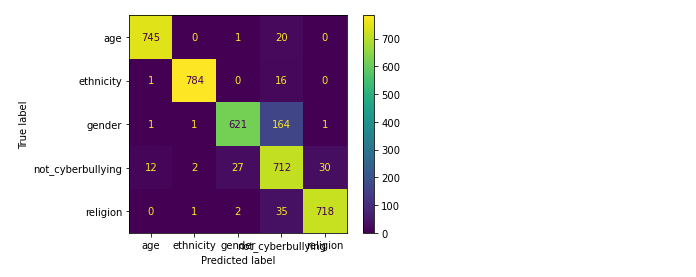
做完数据预处理和特征提取之后需要进一步利用算法来进行结果预测，通过混淆矩阵和分类报告的对比选择最优算法，从而保障数据的精准度。

本次采用了LOGISTIC回归、支持向量机、神经网络、随机森林、提督提升、朴素贝叶斯来进行本次的算法模型，对特定属性：年龄、种族、性别、宗教或其他网络欺凌进行分类分析，本次分析使用了精确率(precision)、召回率(recall)、F1 Score等指标,从而更好的对数据进行精准度的对比。

算法用到的可视化工具为混淆矩阵，用5行5列的矩阵形式来表示。具体评价指标有总体精度、制图精度、用户精度等，这些精度指标从不同的侧面反映了网络欺凌分类的精度。

(1).LOGISTIC回归

from sklearn.experimental import enable_halving_search_cv
from sklearn.model_selection import HalvingGridSearchCV
log_model = LogisticRegression(solver = 'saga')
param_grid = {'C': np.logspace(0, 10, 5)}
grid_log_model = HalvingGridSearchCV(log_model, param_grid = param_grid, n_jobs = -1, min_resources = 'exhaust', factor = 3)
grid_log_model.fit(X_train_tfidf, y_train)
preds_grid_log_model = grid_log_model.predict(X_test_tfidf)
print(classification_report(y_test, preds_grid_log_model))
plot_confusion_matrix(grid_log_model, X_test_tfidf, y_test)

(2).支持向量机

from sklearn.svm import LinearSVC
svm_model = LinearSVC()
C = [1e-5, 1e-4, 1e-2, 1e-1, 1]
param_grid = {'C': C}
grid_svm_model = HalvingGridSearchCV(svm_model, param_grid = param_grid, n_jobs = -1, min_resources = 'exhaust', factor = 3)
grid_svm_model.fit(X_train_tfidf, y_train)
preds_grid_svm_model = grid_svm_model.predict(X_test_tfidf)
print(classification_report(y_test, preds_grid_svm_model))
plot_confusion_matrix(grid_svm_model, X_test_tfidf, y_test)

(3).神经网络

from sklearn.neural_network import MLPClassifier
nn_model = MLPClassifier(activation = 'logistic', max_iter = 10)  # Sigmoid Activation Function
param_grid = {'learning_rate_init': [0.001, 0.0015, 0.002, 0.0025]}
grid_nn_model = HalvingGridSearchCV(nn_model, param_grid = param_grid, n_jobs = -1, min_resources = 'exhaust', factor = 3)
grid_nn_model.fit(X_train_tfidf, y_train)
preds_grid_nn_model = grid_nn_model.predict(X_test_tfidf)
print(classification_report(y_test, preds_grid_nn_model))
plot_confusion_matrix(grid_nn_model, X_test_tfidf, y_test)

(4).随机森林

from sklearn.ensemble import RandomForestClassifier
rf_model = RandomForestClassifier(random_state = 42)
n_estimators = [64, 100, 128]
bootstrap = [True, False] # Bootstrapping is true by default
param_grid = {'n_estimators': n_estimators, 'bootstrap': bootstrap}
grid_rf_model = HalvingGridSearchCV(rf_model, param_grid = param_grid, n_jobs = -1, min_resources = 'exhaust', factor = 3)
grid_rf_model.fit(X_train_tfidf, y_train)
preds_grid_rf_model = grid_rf_model.predict(X_test_tfidf)
print(classification_report(y_test, preds_grid_rf_model))
plot_confusion_matrix(grid_rf_model, X_test_tfidf, y_test)

(5).GRADIENT BOOSTING 梯度提升

from sklearn.ensemble import GradientBoostingClassifier
grad_model = GradientBoostingClassifier(random_state = 42)
param_grid = {'n_estimators': [64, 100, 128, 200]}
grid_grad_model = HalvingGridSearchCV(grad_model, param_grid = param_grid, n_jobs = -1, min_resources = 'exhaust', factor = 3)
grid_grad_model.fit(X_train_tfidf, y_train)
preds_grid_grad_model = grid_grad_model.predict(X_test_tfidf)
print(classification_report(y_test, preds_grid_grad_model))
plot_confusion_matrix(grid_grad_model, X_test_tfidf, y_test)

(6).朴素贝叶斯

from sklearn.naive_bayes import MultinomialNB
nb_model = MultinomialNB()
nb_model.fit(X_train_tfidf, y_train)
preds_nb_model = nb_model.predict(X_test_tfidf)
print(classification_report(y_test, preds_nb_model))
plot_confusion_matrix(nb_model, X_test_tfidf, y_test)

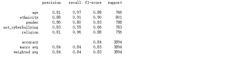
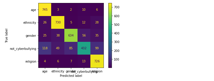
对比上述的混淆矩阵以及分类报告，可看出在相同的数据集的情况下，在上述所尝试的各个模型中随机森林的精确率、召回率、F1-Score均为各模型中精准度最高，所以随机森林模型方法效果最好的。通过文本当中存在的一些敏感单词来检测网络上网络欺凌问题，从而进一步进行屏蔽或封控处理。

4..程序源码

import numpy as np
import pandas as pd
import matplotlib.pyplot as plt
import seaborn as sns
import plotly.express as px
df = pd.read_csv('/Users/xzh/cyberbullying_tweets.csv')  # 导入数据
df.head()
df.info()
pip install demoji
import re
from nltk.corpus import stopwords
from nltk.stem.snowball import SnowballStemmer
import demoji
import string
import warnings
warnings.filterwarnings("ignore")
from warnings import simplefilter
from sklearn.exceptions import ConvergenceWarning
simplefilter("ignore", category=ConvergenceWarning)
STOPWORDS = set(stopwords.words('english'))

STOPWORDS.update(['rt', 'mkr', 'didn', 'bc', 'n', 'm', 
                  'im', 'll', 'y', 've', 'u', 'ur', 'don', 
                  'p', 't', 's', 'aren', 'kp', 'o', 'kat', 
                  'de', 're', 'amp', 'will', 'wa', 'e', 'like'])
stemmer = SnowballStemmer('english')

def clean_text(text):
    
    # 删除标签、提及和URL
    pattern = re.compile(r"(#[A-Za-z0-9]+|@[A-Za-z0-9]+|https?://\S+|www\.\S+|\S+\.[a-z]+|RT @)")
    text = pattern.sub('', text)
    text = " ".join(text.split())
    
    # 使所有文本为小写
    text = text.lower()
    
    
    text = " ".join([stemmer.stem(word) for word in text.split()])
    
    # 删除标点符号
    remove_punc = re.compile(r"[%s]" % re.escape(string.punctuation))
    text = remove_punc.sub('', text)
    
    # 删除停止字
    text = " ".join([word for word in str(text).split() if word not in STOPWORDS])
    
    # 表情符号处理
    emoji = demoji.findall(text)
    for emot in emoji:
        text = re.sub(r"(%s)" % (emot), "_".join(emoji[emot].split()), text)

    return text


 # 将清理函数应用于文本数据

df['cleaned_text'] = df['tweet_text'].apply(lambda text: clean_text(text))



df.head()
df.isnull().sum()  # 查看缺失值
df['cleaned_text'].duplicated().sum() # 查看重复值
df.drop_duplicates("cleaned_text", inplace = True)#去重
df['cleaned_text'].str.isspace().sum()     # 检查只是空格的数据
df = df[df["cyberbullying_type"]!="other_cyberbullying"]
df['cyberbullying_type'].value_counts()#统计类型
sns.countplot(data = df, x = 'cyberbullying_type')
# P绘制每种网络欺凌类型的前15个单词
for cyber_type in df.cyberbullying_type.unique():
    
    top50_word = df.cleaned_text[df.cyberbullying_type==cyber_type].str.split(expand=True).stack().value_counts()[:15]
    
    fig = px.bar(top50_word, color=top50_word.values, color_continuous_scale=px.colors.sequential.RdPu, custom_data=[top50_word.values])
    fig.update_traces(marker_color='red')
    fig.update_traces(hovertemplate='<b>Count: </b>%{customdata[0]}')
    fig.update_layout(title=f"Top 15 words for {cyber_type}",
                     template='simple_white',
                     hovermode='x unified')
    fig.show()
from sklearn.model_selection import train_test_split
from sklearn.feature_extraction.text import TfidfVectorizer
X = df['cleaned_text']  # X
y = df['cyberbullying_type']  # Y
#拆分训练集和测试集
X_train, X_test, y_train, y_test = train_test_split(X, y, test_size = 0.1, random_state = 42)

tfidf = TfidfVectorizer(max_features = 5000)  
#从文本数据中使用TF-IDF矢量器提取前5000个最重要的特征
# 特征提取
X_train_tfidf = tfidf.fit_transform(X_train)  
X_test_tfidf = tfidf.transform(X_test)        
X_train_tfidf  # 创建稀疏矩阵，以节省内存
X_test_tfidf  # 创建稀疏矩阵
from sklearn.preprocessing import StandardScaler
scaler = StandardScaler()
tfidf_array_train = X_train_tfidf.toarray()   # 将稀疏矩阵转换为numpy阵列（密集矩阵）
tfidf_array_test = X_test_tfidf.toarray()     # 
scaled_X_train = scaler.fit_transform(tfidf_array_train)  # 
scaled_X_test = scaler.transform(tfidf_array_test) # 转换训练和测试数据
# 使用主成分分析进行降维
from sklearn.decomposition import PCA
NUM_COMPONENTS = 5000  # 特征总数
pca = PCA(NUM_COMPONENTS)
reduced = pca.fit(scaled_X_train)
variance_explained = np.cumsum(pca.explained_variance_ratio_)  # 计算各分量的累计解释方差
# 画图
fig, ax = plt.subplots(figsize=(8, 6))
plt.plot(range(NUM_COMPONENTS),variance_explained, color='r')
ax.grid(True)
plt.xlabel("Number of components")
plt.ylabel("Cumulative explained variance")
final_pca = PCA(0.9)   
reduced_90 = final_pca.fit_transform(scaled_X_train) # 解释训练数据中90%差异的组件数量

reduced_90_test = final_pca.transform(scaled_X_test)
reduced_90.shape
final_pca = PCA(0.8)
reduced_80 = final_pca.fit_transform(scaled_X_train) # 解释训练数据中80%差异的组件数量
reduced_80.shape
from sklearn.metrics import plot_confusion_matrix, classification_report
# 具有90%方差数据的LOGISTIC回归
from sklearn.linear_model import LogisticRegression
log_model_pca = LogisticRegression()
log_model_pca.fit(reduced_90, y_train)
preds_log_model_pca = log_model_pca.predict(reduced_90_test)
print(classification_report(y_test, preds_log_model_pca))
plot_confusion_matrix(log_model_pca, reduced_90_test, y_test)
# 完整数据的LOGISTIC回归
from sklearn.experimental import enable_halving_search_cv
from sklearn.model_selection import HalvingGridSearchCV
log_model = LogisticRegression(solver = 'saga')
param_grid = {'C': np.logspace(0, 10, 5)}
grid_log_model = HalvingGridSearchCV(log_model, param_grid = param_grid, n_jobs = -1, min_resources = 'exhaust', factor = 3)
grid_log_model.fit(X_train_tfidf, y_train)
preds_grid_log_model = grid_log_model.predict(X_test_tfidf)
print(classification_report(y_test, preds_grid_log_model))
plot_confusion_matrix(grid_log_model, X_test_tfidf, y_test)

grid_log_model.best_estimator_ # C = 1
# 支持向量机
from sklearn.svm import LinearSVC
svm_model = LinearSVC()
C = [1e-5, 1e-4, 1e-2, 1e-1, 1]
param_grid = {'C': C}
grid_svm_model = HalvingGridSearchCV(svm_model, param_grid = param_grid, n_jobs = -1, min_resources = 'exhaust', factor = 3)
grid_svm_model.fit(X_train_tfidf, y_train)
preds_grid_svm_model = grid_svm_model.predict(X_test_tfidf)
print(classification_report(y_test, preds_grid_svm_model))
plot_confusion_matrix(grid_svm_model, X_test_tfidf, y_test)

grid_svm_model.best_estimator_
# 神经网络
from sklearn.neural_network import MLPClassifier
nn_model = MLPClassifier(activation = 'logistic', max_iter = 10)  # Sigmoid Activation Function
param_grid = {'learning_rate_init': [0.001, 0.0015, 0.002, 0.0025]}
grid_nn_model = HalvingGridSearchCV(nn_model, param_grid = param_grid, n_jobs = -1, min_resources = 'exhaust', factor = 3)
grid_nn_model.fit(X_train_tfidf, y_train)
preds_grid_nn_model = grid_nn_model.predict(X_test_tfidf)
print(classification_report(y_test, preds_grid_nn_model))
plot_confusion_matrix(grid_nn_model, X_test_tfidf, y_test)

grid_nn_model.best_estimator_
# 随机森林
from sklearn.ensemble import RandomForestClassifier
rf_model = RandomForestClassifier(random_state = 42)
n_estimators = [64, 100, 128]
bootstrap = [True, False] # Bootstrapping is true by default
param_grid = {'n_estimators': n_estimators, 'bootstrap': bootstrap}
grid_rf_model = HalvingGridSearchCV(rf_model, param_grid = param_grid, n_jobs = -1, min_resources = 'exhaust', factor = 3)
grid_rf_model.fit(X_train_tfidf, y_train)
preds_grid_rf_model = grid_rf_model.predict(X_test_tfidf)
print(classification_report(y_test, preds_grid_rf_model))
plot_confusion_matrix(grid_rf_model, X_test_tfidf, y_test)

grid_rf_model.best_estimator_
#GRADIENT BOOSTING 梯度提升
from sklearn.ensemble import GradientBoostingClassifier
grad_model = GradientBoostingClassifier(random_state = 42)
param_grid = {'n_estimators': [64, 100, 128, 200]}
grid_grad_model = HalvingGridSearchCV(grad_model, param_grid = param_grid, n_jobs = -1, min_resources = 'exhaust', factor = 3)
grid_grad_model.fit(X_train_tfidf, y_train)
preds_grid_grad_model = grid_grad_model.predict(X_test_tfidf)
print(classification_report(y_test, preds_grid_grad_model))
plot_confusion_matrix(grid_grad_model, X_test_tfidf, y_test)

grid_grad_model.best_estimator_
# 朴素贝叶斯
from sklearn.naive_bayes import MultinomialNB
nb_model = MultinomialNB()
nb_model.fit(X_train_tfidf, y_train)
preds_nb_model = nb_model.predict(X_test_tfidf)
print(classification_report(y_test, preds_nb_model))
plot_confusion_matrix(nb_model, X_test_tfidf, y_test)

四、总结

随着网络科技的发展，网络已经成为了我们的聊天工具之一，网络当中的欺凌言论也严重影响着人们的心理健康。如何准确高效的从社交平台言论中检测出欺凌言论是非常具有重要研究意义。为此在此次项目中，运用了公开数据集的数据，利用机器学习的技术对当前已有文本数据准确的将文本中存在的一些单词来检测网络上的网络欺凌问题。根据算法得出的结果可进一步的对一些欺凌字眼进行屏蔽或更进一步的管控措施。

通过此次分析网络上欺凌问题还是普遍存在，尽管算出随机森林算法更精准，但网络言论“缺乏上下文、噪声多、文本短” 等特点，欺凌文本发布者为了避免系统检测，往往会通过人为的方式对关键词进行变形处理，导致其难以取得较好的检测结果，所以后续还得继续提高检测技术，进而提高检测准确率。

在此次课程设计中通过所学到的专业知识和查阅资料后完成数据分析，在遇到困难时我通过网络查询资料以及同学们讨论解决了困难，希望自己可以在不断得加强学习中掌握相关的技能。

posted @ 2022-12-21 23:23 小猪不是佩奇阅读(676) 评论(0) 收藏举报

刷新页面返回顶部