python数据分析第二版:numpy
一:Numpy
# 数组和列表的效率问题,谁优谁劣

# 1.循环遍历
import numpy as np
import time
my_arr = np.arange(1000000)
my_list = list(range(1000000))

def arr_time(array):
    s = time.time()
    for _ in array:
        _ * 2
    e = time.time()
    return e - s

def list_time(list):
    s = time.time()
    for _ in list:
        _ * 2
    e = time.time()
    return e - s

ret1 = arr_time(my_arr)
print("数组运行的时间是{}".format(ret1))
ret2 = list_time(my_list)
print("列表运行的时间是{}".format(ret2))

# 结果
数组运行的时间是0.2110121250152588   # 遍历,列表快
列表运行的时间是0.04800271987915039

# 2.自身扩容
import numpy as np
import time

my_arr = np.arange(1000000)
my_list = list(range(1000000))

def arr_time(array):
    s = time.time()
    for _ in range(10):
        array * 2
    e = time.time()
    return e - s

def list_time(list):
    s = time.time()
    for _ in range(10):
        list * 2
    e = time.time()
    return e - s

ret1 = arr_time(my_arr)
print("数组运行的时间是{}".format(ret1))
ret2 = list_time(my_list)
print("列表运行的时间是{}".format(ret2))
# 结果
数组运行的时间是0.018001317977905273  # 扩容,数组快
列表运行的时间是0.2950167655944824
numpy处理数据快的原因是:在一个连续的内存块中取存取数据。
1. numpy中的ndarray:一种多维的数组对象,是一种快速灵活的大数据容器。
创建ndarray:数组的创建最简单的办法就是使用array函数,它接收一切序列型的对象,其中也包括数组。
data = [1,2,3,4,5]
arr1 = np.array(data)
print(arr1)
# [1,2,3,4,5]  将python的列表,转成数组
data = [[1,2,3,4,5],[6,7,8,9,10]]
arr2 = np.array(data)
print(arr2)

[[ 1  2  3  4  5]
 [ 6  7  8  9 10]]
查看数组的维度和形状
w1 = arr1.ndim  # 维度
s1 = arr1.shape # 形状
w2 = arr2.ndim
s2 = arr2.shape
print("数组arr1的维度是{},形状是{}".format(w1,s1))
print("数组arr2的维度是{},形状是{}".format(w2,s2))
数组arr1的维度是1,形状是(5,)
数组arr2的维度是2,形状是(2, 5)
其他形式的创建数组
np.zeros(20)

# 结果
array([0., 0., 0., 0., 0., 0., 0., 0., 0., 0., 0., 0., 0., 0., 0., 0., 0.,
       0., 0., 0.])

np.zeros((3,6))

# 结果
array([[0., 0., 0., 0., 0., 0.],
       [0., 0., 0., 0., 0., 0.],
       [0., 0., 0., 0., 0., 0.]])

np.ones(10)
array([1., 1., 1., 1., 1., 1., 1., 1., 1., 1.])

np.ones((3,6))
array([[1., 1., 1., 1., 1., 1.],
       [1., 1., 1., 1., 1., 1.],
       [1., 1., 1., 1., 1., 1.]])
np.arrange(10)是python中range的数组版本
np.arange(10)
#
array([0, 1, 2, 3, 4, 5, 6, 7, 8, 9])

2 numpy中的ndarray的数据类型
创建时候指定数据类型
data = [1,2,3,4,5]
arr3 = np.array(data,dtype=np.float64)
print(arr3.dtype)
#
float64
数组数据类型转换
data = [1,2,3,4,5]
arr4 = np.array(data)
print(arr4.dtype)
# int32
float_arr4 = arr4.astype(np.float64)
print(float_arr4.dtype)
# float64
注意:浮点型,转为整形,小数点后面的数组,自动去除,类型与python中的取整。
data = [1.1,2,1,3,1,4,1]
arr5 = np.array(data)
print(arr5.dtype)
int_arr5 = arr5.astype(np.int32)
print(int_arr5.dtype)
#
float64
int32
print(int_arr5)
#
[1 2 1 3 1 4 1]
注意:astype可以将某些全是数值类型的字符串转成数值形式 str = "123456"
demo = ["1","2","3"]
demo_str = np.array(data)
new_demo = demo_str.astype(float)
new_demo
#
array([1.1, 2. , 1. , 3. , 1. , 4. , 1. ])  # 结果很奇怪
二:numpy数组的运算
加减乘除
arr6 = np.array([[1,2,3,4,5],[6,7,8,9,10]])
arr6

# 结果
array([[ 1,  2,  3,  4,  5],
       [ 6,  7,  8,  9, 10]])

arr6 + arr6

# 结果
array([[ 2,  4,  6,  8, 10],
       [12, 14, 16, 18, 20]])

arr6 - arr6

# 结果
array([[0, 0, 0, 0, 0],
       [0, 0, 0, 0, 0]])

arr6 * arr6

# 结果
array([[  1,   4,   9,  16,  25],
       [ 36,  49,  64,  81, 100]])

1 / arr6

# 结果
array([[1.        , 0.5       , 0.33333333, 0.25      , 0.2       ],
       [0.16666667, 0.14285714, 0.125     , 0.11111111, 0.1       ]])
数组之间的比值,产生布尔数组
arr6
array([[ 1,  2,  3,  4,  5],
       [ 6,  7,  8,  9, 10]])

arr7 = np.array([[5,4,1,2,3],[6,8,10,9,7]])
arr7

array([[ 5,  4,  1,  2,  3],
       [ 6,  8, 10,  9,  7]])


arr6 > arr7

# 结果
array([[False, False,  True,  True,  True],
       [False, False, False, False,  True]])
# 数组与常量进行加减乘除,或者数组之间的比较,叫做广播
切片和索引
一维数组的切片和索引
# 一维数组的索引和切片  非常类似于python列表的操作
arr1 = np.arange(10)
arr1
array([0, 1, 2, 3, 4, 5, 6, 7, 8, 9])
arr1[0]
0
arr1[0:-1]
array([0, 1, 2, 3, 4, 5, 6, 7, 8])
注意:不同于列表的地方是:
arr1[:] = 0  # 可以对切片进行改值,将范围内的所有元素改成统一值
arr1
array([0, 0, 0, 0, 0, 0, 0, 0, 0, 0])
arr_slice = arr1[1:3]
arr_slice
array([0, 0])
arr_slice[0] = 1   # 切片不是python字典中的浅拷贝,切片后的元素也是映射到源数组,因此改变切片的内容,也会影响源数组的内容
arr1
array([0, 1, 0, 0, 0, 0, 0, 0, 0, 0])
注意:虽然会影响到源数组,通过复制切片,再进行修改就不会影响到源数组。
arr_slice2 = arr1[1:3].copy()
arr_slice2
array([1, 0])
arr_slice2[0] = 100
arr1
array([0, 1, 0, 0, 0, 0, 0, 0, 0, 0])
高维数组的切片和索引:高维数组的索引,不在是数,而是一个数组
二维数组
arr2 = np.array([[1,3],[2,4]])
arr2
array([[1, 3],
       [2, 4]])
arr2[0]
array([1, 3])
arr2[1]
array([2, 4])
arr2[1][0]
2
arr2[1][1]
4
三维数组
arr3 = np.array([[[1,2,1],[3,4,3],[5,6,5]]])
arr3

array([[[1, 2, 1],
        [3, 4, 3],
        [5, 6, 5]]])

arr3[0]

array([[1, 2, 1],
       [3, 4, 3],
       [5, 6, 5]])

arr3[1]
---------------------------------------------------------------------------
IndexError                                Traceback (most recent call last)
<ipython-input-100-cac0cac14f9a> in <module>
----> 1 arr3[1]

IndexError: index 1 is out of bounds for axis 0 with size 1

# 因为arr3不是这种结构[[  [],[],[]  ],[ [],[],[] ],[ [],[],[] ],[ [],[],[] ]]
arr3[0] 只能取,第一个二维索引,arr3中也只有一个二维索引,1会越界。
注意:arr3[0] 可以用标量和数组进行赋值
arr3[0] = 1
arr3
array([[[1, 1, 1],
        [1, 1, 1],
        [1, 1, 1]]])
arr3[0] = [[0,0,0],[0,0,0],[0,0,0]]
arr3
array([[[0, 0, 0],
        [0, 0, 0],
        [0, 0, 0]]])
注意:三维数组的连续索引
arr3[0][1]
array([0, 0, 0])

arr3[0,1]  # 等价于上面一个
array([0, 0, 0])
二维数组的切片
arr = np.array([[1,2,3],[4,5,6],[7,8,9],[9,8,7],[6,5,4],[3,2,1]])
arr
array([[1, 2, 3],
       [4, 5, 6],
       [7, 8, 9],
       [9, 8, 7],
       [6, 5, 4],
       [3, 2, 1]])

arr[:3]  # 这种形式的切片是按照x,也就是行,进行切片的。

array([[1, 2, 3],
       [4, 5, 6],
       [7, 8, 9]])
arr = np.array([[1,2,3],[4,5,6],[7,8,9],[9,8,7],[6,5,4],[3,2,1]])
arr
array([[1, 2, 3],
       [4, 5, 6],
       [7, 8, 9],
       [9, 8, 7],
       [6, 5, 4],
       [3, 2, 1]])

arr[:3]

array([[1, 2, 3],
       [4, 5, 6],
       [7, 8, 9]])

# 连续按照x轴,即行进行切,第二次切是对每一个一维数组进行切片。

arr[:3,1:]
array([[2, 3],
       [5, 6],
       [8, 9]])
二维数组来说切片 [控制行,控制列]
import numpy as np
import time
arr1 = np.array([[1,2,3],[4,5,6],[7,8,9]])
arr1[1,:2]  # 第二行的前两列
#结果
array([4, 5])
arr1[:2,2]  # 第三列的前两行
#结果
array([3, 6])
arr1 = np.array([[1,2,3],[4,5,6],[7,8,9]])
arr1[:,1:]  # 所有行的第一列之后的所有  :表示所有
# 结果
array([[2, 3],
       [5, 6],
       [8, 9]])
arr1[1:,:] # 所有列的第一行到所有
# 结果
array([[4, 5, 6],
       [7, 8, 9]])
二维切片的赋值也会广播到所有元素
arr1[1:,:] = 100
arr1
# 结果
array([[  1,   2,   3],
       [100, 100, 100],
       [100, 100, 100]])
布尔值索引
arr1 = np.array(["a","b","c","d","e","f","h"])
arr1
# 结果
array(['a', 'b', 'c', 'd', 'e', 'f', 'h'], dtype='<U1')

data = np.random.randn(7,4)  # 生成指定维度的列表,randn函数返回一个或一组样本,具有标准正态分布
data

# 结果
array([[ 0.58942085, -0.68523013, -0.5892267 , -0.97875538],
       [ 0.15429648,  1.56280897,  1.71407167, -0.91513437],
       [ 1.88318536, -1.04312503,  0.22774029,  0.72447885],
       [-0.14408123,  0.0250038 ,  0.47380685,  1.67780702],
       [-0.85254544,  0.6399932 , -0.63439896,  3.21059215],
       [ 0.82560976,  0.84780371,  1.34085735, -0.54620446],
       [ 0.60466595,  0.64945024, -0.76053927, -0.4420415 ]])

arr1 == "a"
#结果
array([ True, False, False, False, False, False, False])

data[arr1=="a"]
# 结果
array([[ 0.58942085, -0.68523013, -0.5892267 , -0.97875538]])  # 第一个为True,所以只显示第一行
关于np.random随机生成数组的其他用法
np.random.rand(4,3,2)   # 生成三维数组,4---包含四行,每行都是一个二维数组,3---包含三行,每个二维数组都是由三行一维数组组成,2---每个一维数组,包含二行,即二个元素。

# 结果
array([[[0.45843663, 0.30801374],
        [0.50365738, 0.49775572],
        [0.86671448, 0.83116069]],

       [[0.26553277, 0.06815584],
        [0.72355103, 0.65145712],
        [0.18559103, 0.77389285]],

       [[0.59710693, 0.4073068 ],
        [0.13812524, 0.16268339],
        [0.92289371, 0.45529381]],

       [[0.51111361, 0.63368562],
        [0.93192965, 0.08373171],
        [0.97425054, 0.53798492]]])

np.random.rand(4,3,3)

# 结果
array([[[0.66847835, 0.96393834, 0.68099953],
        [0.27228911, 0.01407302, 0.1067194 ],
        [0.62624735, 0.58379371, 0.85244324]],

       [[0.15541881, 0.66438894, 0.92232019],
        [0.26811429, 0.13868821, 0.50579811],
        [0.55399624, 0.12154676, 0.06532324]],

       [[0.21546971, 0.10701104, 0.98175299],
        [0.5240603 , 0.58015531, 0.65979757],
        [0.4755814 , 0.34118265, 0.93017974]],

       [[0.87136945, 0.8724195 , 0.13122896],
        [0.84908535, 0.50701899, 0.24765703],
        [0.28119896, 0.76037353, 0.94389406]]])
data[arr1!="a"]
# 结果
array([[ 0.15429648,  1.56280897,  1.71407167, -0.91513437],
       [ 1.88318536, -1.04312503,  0.22774029,  0.72447885],
       [-0.14408123,  0.0250038 ,  0.47380685,  1.67780702],
       [-0.85254544,  0.6399932 , -0.63439896,  3.21059215],
       [ 0.82560976,  0.84780371,  1.34085735, -0.54620446],
       [ 0.60466595,  0.64945024, -0.76053927, -0.4420415 ]])
~非得意思:cont = arr1 == "a" ~cont就是条件取反的意思
cont = arr1 != "a"
data[cont]
# 结果
array([[ 0.15429648,  1.56280897,  1.71407167, -0.91513437],
       [ 1.88318536, -1.04312503,  0.22774029,  0.72447885],
       [-0.14408123,  0.0250038 ,  0.47380685,  1.67780702],
       [-0.85254544,  0.6399932 , -0.63439896,  3.21059215],
       [ 0.82560976,  0.84780371,  1.34085735, -0.54620446],
       [ 0.60466595,  0.64945024, -0.76053927, -0.4420415 ]])

data[~cont]
# 结果
array([[ 0.58942085, -0.68523013, -0.5892267 , -0.97875538]])
布尔值的用处
1.让整个数组里面所有小于0的元素全部变成0
data

# 结果
array([[ 0.58942085, -0.68523013, -0.5892267 , -0.97875538],
       [ 0.15429648,  1.56280897,  1.71407167, -0.91513437],
       [ 1.88318536, -1.04312503,  0.22774029,  0.72447885],
       [-0.14408123,  0.0250038 ,  0.47380685,  1.67780702],
       [-0.85254544,  0.6399932 , -0.63439896,  3.21059215],
       [ 0.82560976,  0.84780371,  1.34085735, -0.54620446],
       [ 0.60466595,  0.64945024, -0.76053927, -0.4420415 ]])


data[data<0] =0
data

# 结果
array([[0.58942085, 0.        , 0.        , 0.        ],
       [0.15429648, 1.56280897, 1.71407167, 0.        ],
       [1.88318536, 0.        , 0.22774029, 0.72447885],
       [0.        , 0.0250038 , 0.47380685, 1.67780702],
       [0.        , 0.6399932 , 0.        , 3.21059215],
       [0.82560976, 0.84780371, 1.34085735, 0.        ],
       [0.60466595, 0.64945024, 0.        , 0.        ]])
&和的意思,类似于and:
data
# 结果
array([[ 0.58942085, -0.68523013, -0.5892267 , -0.97875538],
       [ 0.15429648,  1.56280897,  1.71407167, -0.91513437],
       [ 1.88318536, -1.04312503,  0.22774029,  0.72447885],
       [-0.14408123,  0.0250038 ,  0.47380685,  1.67780702],
       [-0.85254544,  0.6399932 , -0.63439896,  3.21059215],
       [ 0.82560976,  0.84780371,  1.34085735, -0.54620446],
       [ 0.60466595,  0.64945024, -0.76053927, -0.4420415 ]])

# 将里面大于0小于1的数字变成0

data[(data>0) & (data<1)] = 0
data

# 结果
array([[0.        , 0.        , 0.        , 0.        ],
       [0.        , 1.56280897, 1.71407167, 0.        ],
       [1.88318536, 0.        , 0.        , 0.        ],
       [0.        , 0.        , 0.        , 1.67780702],
       [0.        , 0.        , 0.        , 3.21059215],
       [0.        , 0.        , 1.34085735, 0.        ],
       [0.        , 0.        , 0.        , 0.        ]])
| 或的意思,类似于 or
data

# 结果
array([[ 0.58942085, -0.68523013, -0.5892267 , -0.97875538],
       [ 0.15429648,  1.56280897,  1.71407167, -0.91513437],
       [ 1.88318536, -1.04312503,  0.22774029,  0.72447885],
       [-0.14408123,  0.0250038 ,  0.47380685,  1.67780702],
       [-0.85254544,  0.6399932 , -0.63439896,  3.21059215],
       [ 0.82560976,  0.84780371,  1.34085735, -0.54620446],
       [ 0.60466595,  0.64945024, -0.76053927, -0.4420415 ]])

将小于0或者大于1的数修改为1

data[(data<0) | (data>1)] = 1
data
# 结果
array([[1.        , 1.        , 0.59208795, 1.        ],
       [1.        , 1.        , 1.        , 1.        ],
       [1.        , 0.0701599 , 1.        , 0.15396346],
       [1.        , 1.        , 1.        , 0.2735209 ],
       [1.        , 1.        , 1.        , 1.        ],
       [1.        , 1.        , 1.        , 0.06469213],
       [1.        , 1.        , 1.        , 1.        ]])
花式索引
np.empty()返回一个随机元素的矩阵,大小按照参数定义。不是字面意思上的空数组,需要自己调整参数。
data = np.empty((8,4))  # 本意想生成8行4列的二维空数组
data
# 结果
array([[9.34e-322, 0.00e+000, 0.00e+000, 0.00e+000],
       [0.00e+000, 0.00e+000, 0.00e+000, 0.00e+000],
       [0.00e+000, 0.00e+000, 0.00e+000, 0.00e+000],
       [0.00e+000, 0.00e+000, 0.00e+000, 0.00e+000],
       [0.00e+000, 0.00e+000, 0.00e+000, 0.00e+000],
       [0.00e+000, 0.00e+000, 0.00e+000, 0.00e+000],
       [0.00e+000, 0.00e+000, 0.00e+000, 0.00e+000],
       [0.00e+000, 0.00e+000, 0.00e+000, 0.00e+000]])

# 空数组需要手动调整

for i in range(8):
    data[i] = 0

data

#结果
array([[0., 0., 0., 0.],
       [0., 0., 0., 0.],
       [0., 0., 0., 0.],
       [0., 0., 0., 0.],
       [0., 0., 0., 0.],
       [0., 0., 0., 0.],
       [0., 0., 0., 0.],
       [0., 0., 0., 0.]])
索引数组:按照顺序返回结果
for i in range(8):
    data[i] = i

data
# 结果

array([[0., 0., 0., 0.],
       [1., 1., 1., 1.],
       [2., 2., 2., 2.],
       [3., 3., 3., 3.],
       [4., 4., 4., 4.],
       [5., 5., 5., 5.],
       [6., 6., 6., 6.],
       [7., 7., 7., 7.]])

# 按照顺序取出,每一行
data[[0,2,4,6]]   data[[索引值]]
# 结果
array([[0., 0., 0., 0.],
       [2., 2., 2., 2.],
       [4., 4., 4., 4.],
       [6., 6., 6., 6.]])
# 另一种方式
data[[i for i in range(len(data)) if i % 2 == 0]]
data
# 结果
array([[0., 0., 0., 0.],
[2., 2., 2., 2.],
[4., 4., 4., 4.],
[6., 6., 6., 6.]])
多个索引数组:以二维为例,返回的是一个一维数组
data = np.arange(32)
data
array([ 0,  1,  2,  3,  4,  5,  6,  7,  8,  9, 10, 11, 12, 13, 14, 15, 16,
       17, 18, 19, 20, 21, 22, 23, 24, 25, 26, 27, 28, 29, 30, 31])
data = data.reshape(8,4)
data
array([[ 0,  1,  2,  3],
       [ 4,  5,  6,  7],
       [ 8,  9, 10, 11],
       [12, 13, 14, 15],
       [16, 17, 18, 19],
       [20, 21, 22, 23],
       [24, 25, 26, 27],
       [28, 29, 30, 31]])
data[[0,2,4,6],[3,2,1,0]]
array([ 3, 10, 17, 24])
# 二维最终选出的数其实是 (0,3),(2,2),(4,1),(6,0)组成的一维数组
数组的转置
data = np.arange(15).reshape(3,5)
data
# 结果
array([[ 0,  1,  2,  3,  4],
       [ 5,  6,  7,  8,  9],
       [10, 11, 12, 13, 14]])

data.T
array([[ 0,  5, 10],
       [ 1,  6, 11],
       [ 2,  7, 12],
       [ 3,  8, 13],
       [ 4,  9, 14]])

行变成列或列变行
矩阵的內积,A*A^T
ret1 = np.dot(data,data.T)  3*5, 5*3 --- 3*3
ret1
array([[ 30,  80, 130],   # 30 = (0*0 + 1*1 + 2*2 + 3*3 + 4*4)
       [ 80, 255, 430],
       [130, 430, 730]])
ret2 = np.dot(data.T,data)  5*3 , 3*5 --- 5*5   # 內积的正确方法
ret2
array([[125, 140, 155, 170, 185],
       [140, 158, 176, 194, 212],
       [155, 176, 197, 218, 239],
       [170, 194, 218, 242, 266],
       [185, 212, 239, 266, 293]])
高维数组的轴对换
data = np.arange(16).reshape((2,2,4))
data
# 结果
array([[[ 0,  1,  2,  3],
        [ 4,  5,  6,  7]],

       [[ 8,  9, 10, 11],
        [12, 13, 14, 15]]])

data.transpose((1,0,2))
data
# 结果
array([[[ 0,  1,  2,  3],
        [ 8,  9, 10, 11]],

       [[ 4,  5,  6,  7],
        [12, 13, 14, 15]]])

解析:其中正确的应该是(0,1,2)分别表示(x,y,z)(1,0,2)表明x轴和y轴进行了调换

那么导致索引值变化:
data[0,0] --->data[0,0]
data[0,1] --->data[1,0]
data[1,0] --->data[0,1]
data[1,1] --->data[1,1]

data.transpose((2,1,0)) 表示x轴和z轴进行了变换。
x轴和z后就牵扯到结构的变化和,原来的结构是2*2*4--二行二维数组,每个二维数组里面有两行一维数组,每个一维数组里面有四行数据。

(2,2, 4) 的结构变成了 (4, 2, 2)

[
[[],[]],
[[],[]],
[[],[]],
[[],[]],

]

结构变化后,然后开始赋值,data[0][1][1]  = 5变成了 data[1][1][0]  = 5

[
[[],[]],
[[],[5]],
[[],[]],
[[],[]],

]
原来的data[1][1][0] = 12 变成了 data[0][1][1] = 12

[
[[],[12]],
[[],[5]],
[[],[]],
[[],[]],
]
以此类推的出变化后的值

array([[[ 0,  1],
        [ 2,  3]],

       [[ 4,  5],
        [ 6,  7]],

       [[ 8,  9],
        [10, 11]],

       [[12, 13],
        [14, 15]]])

总结:和Z轴相关的变换都需换换结构,然后在改变索引值。
swapaxes的轴对换:简写模式 swapaxes(1,2) 就是y轴和z轴进行变换。data[0][1][0]的值就变成data[0][0][1]的值
data = np.arange(0,16).reshape(2,2,4)
data
# 结果
array([[[ 0,  1,  2,  3],
        [ 4,  5,  6,  7]],

       [[ 8,  9, 10, 11],
        [12, 13, 14, 15]]])

data.swapaxes(1,2)
# 结果
array([[[ 0,  4],
        [ 1,  5],
        [ 2,  6],
        [ 3,  7]],

       [[ 8, 12],
        [ 9, 13],
        [10, 14],
        [11, 15]]])

第一步,shape(2,2,4)经过y轴和z轴的变换,形状变成shape(2,4,2)---变形状

【[[],
    [],
    [],
    []],
  [[],
   [],
   [],
   []]】

第二步,值变换,data[0][1][0]的值变成data[0][0][1]的值,经过所有的值变换,得到结果---变值
总结:轴变换的步骤,先根据函数(参数)变形状,然后变值
2.通用函数:快速的元素级数组函数
就是对ndarray的数据进行元素级 操作的函数,接收一个或多个标量值,并返回一个或多个标量值。ufunc
sqrt函数 对每个元素进行二次开方操作 二次根号下
data = np.arange(0,16)
data
# 结果
array([ 0,  1,  2,  3,  4,  5,  6,  7,  8,  9, 10, 11, 12, 13, 14, 15])

np.sqrt(data)
# 结果
array([0.        , 1.        , 1.41421356, 1.73205081, 2.        ,
       2.23606798, 2.44948974, 2.64575131, 2.82842712, 3.        ,
       3.16227766, 3.31662479, 3.46410162, 3.60555128, 3.74165739,
       3.87298335])
exp函数:exp,高等数学里以自然常数e为底的指数函数;Exp:返回e的n次方,e是一个常数为2.71828;Exp 函数 返回 e(自然对数的底)的幂次方。
np.exp(data)
# 结果
array([1.00000000e+00, 2.71828183e+00, 7.38905610e+00, 2.00855369e+01,
       5.45981500e+01, 1.48413159e+02, 4.03428793e+02, 1.09663316e+03,
       2.98095799e+03, 8.10308393e+03, 2.20264658e+04, 5.98741417e+04,
       1.62754791e+05, 4.42413392e+05, 1.20260428e+06, 3.26901737e+06])
二元ufunc:接收两个数组参数
x = np.random.randn(8)
x
# 结果
array([-2.15378687,  0.81808891,  1.03173227, -1.38834899, -0.25440583,
        0.15042907,  0.78186255, -1.56663501])

y = np.random.randn(8)
y
# 结果
array([ 0.99923527, -0.05346302,  0.36369126, -1.14881998,  1.13355945,
        0.37692407, -0.00560708,  0.24598121])

np.maximum(x,y)
# 结果
array([ 0.99923527, -0.05346302,  0.36369126,  1.50986447,  1.32350916,
        0.37692407,  0.13424535,  0.44801383])
# 函数方面未整理完全--TODO
3.利用数据进行数据处理
一般处理数组,需要循环数组,对每个元素进行处理,但是数组表达式可以代替循环的做法
例如:在一组值(网格型)上计算函数sqrt(x^2 + y^2)。np.meshgrid函数接收两个一维数组,并产生两个二维矩阵(对应连个数组中的所有(x,y)对):


import numpy as np
points = np.arange(-5,5,0.01)
points
# 结果
array([-5.0000000e+00, -4.9900000e+00, -4.9800000e+00, -4.9700000e+00,
       -4.9600000e+00, -4.9500000e+00, -4.9400000e+00, -4.9300000e+00,
       -4.9200000e+00, -4.9100000e+00, -4.9000000e+00, -4.8900000e+00,
       -4.8800000e+00, -4.8700000e+00, -4.8600000e+00, -4.8500000e+00,
       -4.8400000e+00, -4.8300000e+00, -4.8200000e+00, -4.8100000e+00,
       -4.8000000e+00, -4.7900000e+00, -4.7800000e+00, -4.7700000e+00,
       -4.7600000e+00, -4.7500000e+00, -4.7400000e+00, -4.7300000e+00,
       -4.7200000e+00, -4.7100000e+00, -4.7000000e+00, -4.6900000e+00,
       -4.6800000e+00, -4.6700000e+00, -4.6600000e+00, -4.6500000e+00,
       -4.6400000e+00, -4.6300000e+00, -4.6200000e+00, -4.6100000e+00,
       -4.6000000e+00, -4.5900000e+00, -4.5800000e+00, -4.5700000e+00,
       -4.5600000e+00, -4.5500000e+00, -4.5400000e+00, -4.5300000e+00,
       -4.5200000e+00, -4.5100000e+00, -4.5000000e+00, -4.4900000e+00,
       -4.4800000e+00, -4.4700000e+00, -4.4600000e+00, -4.4500000e+00,
       -4.4400000e+00, -4.4300000e+00, -4.4200000e+00, -4.4100000e+00,
       -4.4000000e+00, -4.3900000e+00, -4.3800000e+00, -4.3700000e+00,
       -4.3600000e+00, -4.3500000e+00, -4.3400000e+00, -4.3300000e+00,
       -4.3200000e+00, -4.3100000e+00, -4.3000000e+00, -4.2900000e+00,
       -4.2800000e+00, -4.2700000e+00, -4.2600000e+00, -4.2500000e+00,
       -4.2400000e+00, -4.2300000e+00, -4.2200000e+00, -4.2100000e+00,
       -4.2000000e+00, -4.1900000e+00, -4.1800000e+00, -4.1700000e+00,
       -4.1600000e+00, -4.1500000e+00, -4.1400000e+00, -4.1300000e+00,
       -4.1200000e+00, -4.1100000e+00, -4.1000000e+00, -4.0900000e+00,
       -4.0800000e+00, -4.0700000e+00, -4.0600000e+00, -4.0500000e+00,
       -4.0400000e+00, -4.0300000e+00, -4.0200000e+00, -4.0100000e+00,
       -4.0000000e+00, -3.9900000e+00, -3.9800000e+00, -3.9700000e+00,
       -3.9600000e+00, -3.9500000e+00, -3.9400000e+00, -3.9300000e+00,
       -3.9200000e+00, -3.9100000e+00, -3.9000000e+00, -3.8900000e+00,
       -3.8800000e+00, -3.8700000e+00, -3.8600000e+00, -3.8500000e+00,
       -3.8400000e+00, -3.8300000e+00, -3.8200000e+00, -3.8100000e+00,
       -3.8000000e+00, -3.7900000e+00, -3.7800000e+00, -3.7700000e+00,
       -3.7600000e+00, -3.7500000e+00, -3.7400000e+00, -3.7300000e+00,
       -3.7200000e+00, -3.7100000e+00, -3.7000000e+00, -3.6900000e+00,
       -3.6800000e+00, -3.6700000e+00, -3.6600000e+00, -3.6500000e+00,
       -3.6400000e+00, -3.6300000e+00, -3.6200000e+00, -3.6100000e+00,
       -3.6000000e+00, -3.5900000e+00, -3.5800000e+00, -3.5700000e+00,
       -3.5600000e+00, -3.5500000e+00, -3.5400000e+00, -3.5300000e+00,
       -3.5200000e+00, -3.5100000e+00, -3.5000000e+00, -3.4900000e+00,
       -3.4800000e+00, -3.4700000e+00, -3.4600000e+00, -3.4500000e+00,
       -3.4400000e+00, -3.4300000e+00, -3.4200000e+00, -3.4100000e+00,
       -3.4000000e+00, -3.3900000e+00, -3.3800000e+00, -3.3700000e+00,
       -3.3600000e+00, -3.3500000e+00, -3.3400000e+00, -3.3300000e+00,
       -3.3200000e+00, -3.3100000e+00, -3.3000000e+00, -3.2900000e+00,
       -3.2800000e+00, -3.2700000e+00, -3.2600000e+00, -3.2500000e+00,
       -3.2400000e+00, -3.2300000e+00, -3.2200000e+00, -3.2100000e+00,
       -3.2000000e+00, -3.1900000e+00, -3.1800000e+00, -3.1700000e+00,
       -3.1600000e+00, -3.1500000e+00, -3.1400000e+00, -3.1300000e+00,
       -3.1200000e+00, -3.1100000e+00, -3.1000000e+00, -3.0900000e+00,
       -3.0800000e+00, -3.0700000e+00, -3.0600000e+00, -3.0500000e+00,
       -3.0400000e+00, -3.0300000e+00, -3.0200000e+00, -3.0100000e+00,
       -3.0000000e+00, -2.9900000e+00, -2.9800000e+00, -2.9700000e+00,
       -2.9600000e+00, -2.9500000e+00, -2.9400000e+00, -2.9300000e+00,
       -2.9200000e+00, -2.9100000e+00, -2.9000000e+00, -2.8900000e+00,
       -2.8800000e+00, -2.8700000e+00, -2.8600000e+00, -2.8500000e+00,
       -2.8400000e+00, -2.8300000e+00, -2.8200000e+00, -2.8100000e+00,
       -2.8000000e+00, -2.7900000e+00, -2.7800000e+00, -2.7700000e+00,
       -2.7600000e+00, -2.7500000e+00, -2.7400000e+00, -2.7300000e+00,
       -2.7200000e+00, -2.7100000e+00, -2.7000000e+00, -2.6900000e+00,
       -2.6800000e+00, -2.6700000e+00, -2.6600000e+00, -2.6500000e+00,
       -2.6400000e+00, -2.6300000e+00, -2.6200000e+00, -2.6100000e+00,
       -2.6000000e+00, -2.5900000e+00, -2.5800000e+00, -2.5700000e+00,
       -2.5600000e+00, -2.5500000e+00, -2.5400000e+00, -2.5300000e+00,
       -2.5200000e+00, -2.5100000e+00, -2.5000000e+00, -2.4900000e+00,
       -2.4800000e+00, -2.4700000e+00, -2.4600000e+00, -2.4500000e+00,
       -2.4400000e+00, -2.4300000e+00, -2.4200000e+00, -2.4100000e+00,
       -2.4000000e+00, -2.3900000e+00, -2.3800000e+00, -2.3700000e+00,
       -2.3600000e+00, -2.3500000e+00, -2.3400000e+00, -2.3300000e+00,
       -2.3200000e+00, -2.3100000e+00, -2.3000000e+00, -2.2900000e+00,
       -2.2800000e+00, -2.2700000e+00, -2.2600000e+00, -2.2500000e+00,
       -2.2400000e+00, -2.2300000e+00, -2.2200000e+00, -2.2100000e+00,
       -2.2000000e+00, -2.1900000e+00, -2.1800000e+00, -2.1700000e+00,
       -2.1600000e+00, -2.1500000e+00, -2.1400000e+00, -2.1300000e+00,
       -2.1200000e+00, -2.1100000e+00, -2.1000000e+00, -2.0900000e+00,
       -2.0800000e+00, -2.0700000e+00, -2.0600000e+00, -2.0500000e+00,
       -2.0400000e+00, -2.0300000e+00, -2.0200000e+00, -2.0100000e+00,
       -2.0000000e+00, -1.9900000e+00, -1.9800000e+00, -1.9700000e+00,
       -1.9600000e+00, -1.9500000e+00, -1.9400000e+00, -1.9300000e+00,
       -1.9200000e+00, -1.9100000e+00, -1.9000000e+00, -1.8900000e+00,
       -1.8800000e+00, -1.8700000e+00, -1.8600000e+00, -1.8500000e+00,
       -1.8400000e+00, -1.8300000e+00, -1.8200000e+00, -1.8100000e+00,
       -1.8000000e+00, -1.7900000e+00, -1.7800000e+00, -1.7700000e+00,
       -1.7600000e+00, -1.7500000e+00, -1.7400000e+00, -1.7300000e+00,
       -1.7200000e+00, -1.7100000e+00, -1.7000000e+00, -1.6900000e+00,
       -1.6800000e+00, -1.6700000e+00, -1.6600000e+00, -1.6500000e+00,
       -1.6400000e+00, -1.6300000e+00, -1.6200000e+00, -1.6100000e+00,
       -1.6000000e+00, -1.5900000e+00, -1.5800000e+00, -1.5700000e+00,
       -1.5600000e+00, -1.5500000e+00, -1.5400000e+00, -1.5300000e+00,
       -1.5200000e+00, -1.5100000e+00, -1.5000000e+00, -1.4900000e+00,
       -1.4800000e+00, -1.4700000e+00, -1.4600000e+00, -1.4500000e+00,
       -1.4400000e+00, -1.4300000e+00, -1.4200000e+00, -1.4100000e+00,
       -1.4000000e+00, -1.3900000e+00, -1.3800000e+00, -1.3700000e+00,
       -1.3600000e+00, -1.3500000e+00, -1.3400000e+00, -1.3300000e+00,
       -1.3200000e+00, -1.3100000e+00, -1.3000000e+00, -1.2900000e+00,
       -1.2800000e+00, -1.2700000e+00, -1.2600000e+00, -1.2500000e+00,
       -1.2400000e+00, -1.2300000e+00, -1.2200000e+00, -1.2100000e+00,
       -1.2000000e+00, -1.1900000e+00, -1.1800000e+00, -1.1700000e+00,
       -1.1600000e+00, -1.1500000e+00, -1.1400000e+00, -1.1300000e+00,
       -1.1200000e+00, -1.1100000e+00, -1.1000000e+00, -1.0900000e+00,
       -1.0800000e+00, -1.0700000e+00, -1.0600000e+00, -1.0500000e+00,
       -1.0400000e+00, -1.0300000e+00, -1.0200000e+00, -1.0100000e+00,
       -1.0000000e+00, -9.9000000e-01, -9.8000000e-01, -9.7000000e-01,
       -9.6000000e-01, -9.5000000e-01, -9.4000000e-01, -9.3000000e-01,
       -9.2000000e-01, -9.1000000e-01, -9.0000000e-01, -8.9000000e-01,
       -8.8000000e-01, -8.7000000e-01, -8.6000000e-01, -8.5000000e-01,
       -8.4000000e-01, -8.3000000e-01, -8.2000000e-01, -8.1000000e-01,
       -8.0000000e-01, -7.9000000e-01, -7.8000000e-01, -7.7000000e-01,
       -7.6000000e-01, -7.5000000e-01, -7.4000000e-01, -7.3000000e-01,
       -7.2000000e-01, -7.1000000e-01, -7.0000000e-01, -6.9000000e-01,
       -6.8000000e-01, -6.7000000e-01, -6.6000000e-01, -6.5000000e-01,
       -6.4000000e-01, -6.3000000e-01, -6.2000000e-01, -6.1000000e-01,
       -6.0000000e-01, -5.9000000e-01, -5.8000000e-01, -5.7000000e-01,
       -5.6000000e-01, -5.5000000e-01, -5.4000000e-01, -5.3000000e-01,
       -5.2000000e-01, -5.1000000e-01, -5.0000000e-01, -4.9000000e-01,
       -4.8000000e-01, -4.7000000e-01, -4.6000000e-01, -4.5000000e-01,
       -4.4000000e-01, -4.3000000e-01, -4.2000000e-01, -4.1000000e-01,
       -4.0000000e-01, -3.9000000e-01, -3.8000000e-01, -3.7000000e-01,
       -3.6000000e-01, -3.5000000e-01, -3.4000000e-01, -3.3000000e-01,
       -3.2000000e-01, -3.1000000e-01, -3.0000000e-01, -2.9000000e-01,
       -2.8000000e-01, -2.7000000e-01, -2.6000000e-01, -2.5000000e-01,
       -2.4000000e-01, -2.3000000e-01, -2.2000000e-01, -2.1000000e-01,
       -2.0000000e-01, -1.9000000e-01, -1.8000000e-01, -1.7000000e-01,
       -1.6000000e-01, -1.5000000e-01, -1.4000000e-01, -1.3000000e-01,
       -1.2000000e-01, -1.1000000e-01, -1.0000000e-01, -9.0000000e-02,
       -8.0000000e-02, -7.0000000e-02, -6.0000000e-02, -5.0000000e-02,
       -4.0000000e-02, -3.0000000e-02, -2.0000000e-02, -1.0000000e-02,
       -1.0658141e-13,  1.0000000e-02,  2.0000000e-02,  3.0000000e-02,
        4.0000000e-02,  5.0000000e-02,  6.0000000e-02,  7.0000000e-02,
        8.0000000e-02,  9.0000000e-02,  1.0000000e-01,  1.1000000e-01,
        1.2000000e-01,  1.3000000e-01,  1.4000000e-01,  1.5000000e-01,
        1.6000000e-01,  1.7000000e-01,  1.8000000e-01,  1.9000000e-01,
        2.0000000e-01,  2.1000000e-01,  2.2000000e-01,  2.3000000e-01,
        2.4000000e-01,  2.5000000e-01,  2.6000000e-01,  2.7000000e-01,
        2.8000000e-01,  2.9000000e-01,  3.0000000e-01,  3.1000000e-01,
        3.2000000e-01,  3.3000000e-01,  3.4000000e-01,  3.5000000e-01,
        3.6000000e-01,  3.7000000e-01,  3.8000000e-01,  3.9000000e-01,
        4.0000000e-01,  4.1000000e-01,  4.2000000e-01,  4.3000000e-01,
        4.4000000e-01,  4.5000000e-01,  4.6000000e-01,  4.7000000e-01,
        4.8000000e-01,  4.9000000e-01,  5.0000000e-01,  5.1000000e-01,
        5.2000000e-01,  5.3000000e-01,  5.4000000e-01,  5.5000000e-01,
        5.6000000e-01,  5.7000000e-01,  5.8000000e-01,  5.9000000e-01,
        6.0000000e-01,  6.1000000e-01,  6.2000000e-01,  6.3000000e-01,
        6.4000000e-01,  6.5000000e-01,  6.6000000e-01,  6.7000000e-01,
        6.8000000e-01,  6.9000000e-01,  7.0000000e-01,  7.1000000e-01,
        7.2000000e-01,  7.3000000e-01,  7.4000000e-01,  7.5000000e-01,
        7.6000000e-01,  7.7000000e-01,  7.8000000e-01,  7.9000000e-01,
        8.0000000e-01,  8.1000000e-01,  8.2000000e-01,  8.3000000e-01,
        8.4000000e-01,  8.5000000e-01,  8.6000000e-01,  8.7000000e-01,
        8.8000000e-01,  8.9000000e-01,  9.0000000e-01,  9.1000000e-01,
        9.2000000e-01,  9.3000000e-01,  9.4000000e-01,  9.5000000e-01,
        9.6000000e-01,  9.7000000e-01,  9.8000000e-01,  9.9000000e-01,
        1.0000000e+00,  1.0100000e+00,  1.0200000e+00,  1.0300000e+00,
        1.0400000e+00,  1.0500000e+00,  1.0600000e+00,  1.0700000e+00,
        1.0800000e+00,  1.0900000e+00,  1.1000000e+00,  1.1100000e+00,
        1.1200000e+00,  1.1300000e+00,  1.1400000e+00,  1.1500000e+00,
        1.1600000e+00,  1.1700000e+00,  1.1800000e+00,  1.1900000e+00,
        1.2000000e+00,  1.2100000e+00,  1.2200000e+00,  1.2300000e+00,
        1.2400000e+00,  1.2500000e+00,  1.2600000e+00,  1.2700000e+00,
        1.2800000e+00,  1.2900000e+00,  1.3000000e+00,  1.3100000e+00,
        1.3200000e+00,  1.3300000e+00,  1.3400000e+00,  1.3500000e+00,
        1.3600000e+00,  1.3700000e+00,  1.3800000e+00,  1.3900000e+00,
        1.4000000e+00,  1.4100000e+00,  1.4200000e+00,  1.4300000e+00,
        1.4400000e+00,  1.4500000e+00,  1.4600000e+00,  1.4700000e+00,
        1.4800000e+00,  1.4900000e+00,  1.5000000e+00,  1.5100000e+00,
        1.5200000e+00,  1.5300000e+00,  1.5400000e+00,  1.5500000e+00,
        1.5600000e+00,  1.5700000e+00,  1.5800000e+00,  1.5900000e+00,
        1.6000000e+00,  1.6100000e+00,  1.6200000e+00,  1.6300000e+00,
        1.6400000e+00,  1.6500000e+00,  1.6600000e+00,  1.6700000e+00,
        1.6800000e+00,  1.6900000e+00,  1.7000000e+00,  1.7100000e+00,
        1.7200000e+00,  1.7300000e+00,  1.7400000e+00,  1.7500000e+00,
        1.7600000e+00,  1.7700000e+00,  1.7800000e+00,  1.7900000e+00,
        1.8000000e+00,  1.8100000e+00,  1.8200000e+00,  1.8300000e+00,
        1.8400000e+00,  1.8500000e+00,  1.8600000e+00,  1.8700000e+00,
        1.8800000e+00,  1.8900000e+00,  1.9000000e+00,  1.9100000e+00,
        1.9200000e+00,  1.9300000e+00,  1.9400000e+00,  1.9500000e+00,
        1.9600000e+00,  1.9700000e+00,  1.9800000e+00,  1.9900000e+00,
        2.0000000e+00,  2.0100000e+00,  2.0200000e+00,  2.0300000e+00,
        2.0400000e+00,  2.0500000e+00,  2.0600000e+00,  2.0700000e+00,
        2.0800000e+00,  2.0900000e+00,  2.1000000e+00,  2.1100000e+00,
        2.1200000e+00,  2.1300000e+00,  2.1400000e+00,  2.1500000e+00,
        2.1600000e+00,  2.1700000e+00,  2.1800000e+00,  2.1900000e+00,
        2.2000000e+00,  2.2100000e+00,  2.2200000e+00,  2.2300000e+00,
        2.2400000e+00,  2.2500000e+00,  2.2600000e+00,  2.2700000e+00,
        2.2800000e+00,  2.2900000e+00,  2.3000000e+00,  2.3100000e+00,
        2.3200000e+00,  2.3300000e+00,  2.3400000e+00,  2.3500000e+00,
        2.3600000e+00,  2.3700000e+00,  2.3800000e+00,  2.3900000e+00,
        2.4000000e+00,  2.4100000e+00,  2.4200000e+00,  2.4300000e+00,
        2.4400000e+00,  2.4500000e+00,  2.4600000e+00,  2.4700000e+00,
        2.4800000e+00,  2.4900000e+00,  2.5000000e+00,  2.5100000e+00,
        2.5200000e+00,  2.5300000e+00,  2.5400000e+00,  2.5500000e+00,
        2.5600000e+00,  2.5700000e+00,  2.5800000e+00,  2.5900000e+00,
        2.6000000e+00,  2.6100000e+00,  2.6200000e+00,  2.6300000e+00,
        2.6400000e+00,  2.6500000e+00,  2.6600000e+00,  2.6700000e+00,
        2.6800000e+00,  2.6900000e+00,  2.7000000e+00,  2.7100000e+00,
        2.7200000e+00,  2.7300000e+00,  2.7400000e+00,  2.7500000e+00,
        2.7600000e+00,  2.7700000e+00,  2.7800000e+00,  2.7900000e+00,
        2.8000000e+00,  2.8100000e+00,  2.8200000e+00,  2.8300000e+00,
        2.8400000e+00,  2.8500000e+00,  2.8600000e+00,  2.8700000e+00,
        2.8800000e+00,  2.8900000e+00,  2.9000000e+00,  2.9100000e+00,
        2.9200000e+00,  2.9300000e+00,  2.9400000e+00,  2.9500000e+00,
        2.9600000e+00,  2.9700000e+00,  2.9800000e+00,  2.9900000e+00,
        3.0000000e+00,  3.0100000e+00,  3.0200000e+00,  3.0300000e+00,
        3.0400000e+00,  3.0500000e+00,  3.0600000e+00,  3.0700000e+00,
        3.0800000e+00,  3.0900000e+00,  3.1000000e+00,  3.1100000e+00,
        3.1200000e+00,  3.1300000e+00,  3.1400000e+00,  3.1500000e+00,
        3.1600000e+00,  3.1700000e+00,  3.1800000e+00,  3.1900000e+00,
        3.2000000e+00,  3.2100000e+00,  3.2200000e+00,  3.2300000e+00,
        3.2400000e+00,  3.2500000e+00,  3.2600000e+00,  3.2700000e+00,
        3.2800000e+00,  3.2900000e+00,  3.3000000e+00,  3.3100000e+00,
        3.3200000e+00,  3.3300000e+00,  3.3400000e+00,  3.3500000e+00,
        3.3600000e+00,  3.3700000e+00,  3.3800000e+00,  3.3900000e+00,
        3.4000000e+00,  3.4100000e+00,  3.4200000e+00,  3.4300000e+00,
        3.4400000e+00,  3.4500000e+00,  3.4600000e+00,  3.4700000e+00,
        3.4800000e+00,  3.4900000e+00,  3.5000000e+00,  3.5100000e+00,
        3.5200000e+00,  3.5300000e+00,  3.5400000e+00,  3.5500000e+00,
        3.5600000e+00,  3.5700000e+00,  3.5800000e+00,  3.5900000e+00,
        3.6000000e+00,  3.6100000e+00,  3.6200000e+00,  3.6300000e+00,
        3.6400000e+00,  3.6500000e+00,  3.6600000e+00,  3.6700000e+00,
        3.6800000e+00,  3.6900000e+00,  3.7000000e+00,  3.7100000e+00,
        3.7200000e+00,  3.7300000e+00,  3.7400000e+00,  3.7500000e+00,
        3.7600000e+00,  3.7700000e+00,  3.7800000e+00,  3.7900000e+00,
        3.8000000e+00,  3.8100000e+00,  3.8200000e+00,  3.8300000e+00,
        3.8400000e+00,  3.8500000e+00,  3.8600000e+00,  3.8700000e+00,
        3.8800000e+00,  3.8900000e+00,  3.9000000e+00,  3.9100000e+00,
        3.9200000e+00,  3.9300000e+00,  3.9400000e+00,  3.9500000e+00,
        3.9600000e+00,  3.9700000e+00,  3.9800000e+00,  3.9900000e+00,
        4.0000000e+00,  4.0100000e+00,  4.0200000e+00,  4.0300000e+00,
        4.0400000e+00,  4.0500000e+00,  4.0600000e+00,  4.0700000e+00,
        4.0800000e+00,  4.0900000e+00,  4.1000000e+00,  4.1100000e+00,
        4.1200000e+00,  4.1300000e+00,  4.1400000e+00,  4.1500000e+00,
        4.1600000e+00,  4.1700000e+00,  4.1800000e+00,  4.1900000e+00,
        4.2000000e+00,  4.2100000e+00,  4.2200000e+00,  4.2300000e+00,
        4.2400000e+00,  4.2500000e+00,  4.2600000e+00,  4.2700000e+00,
        4.2800000e+00,  4.2900000e+00,  4.3000000e+00,  4.3100000e+00,
        4.3200000e+00,  4.3300000e+00,  4.3400000e+00,  4.3500000e+00,
        4.3600000e+00,  4.3700000e+00,  4.3800000e+00,  4.3900000e+00,
        4.4000000e+00,  4.4100000e+00,  4.4200000e+00,  4.4300000e+00,
        4.4400000e+00,  4.4500000e+00,  4.4600000e+00,  4.4700000e+00,
        4.4800000e+00,  4.4900000e+00,  4.5000000e+00,  4.5100000e+00,
        4.5200000e+00,  4.5300000e+00,  4.5400000e+00,  4.5500000e+00,
        4.5600000e+00,  4.5700000e+00,  4.5800000e+00,  4.5900000e+00,
        4.6000000e+00,  4.6100000e+00,  4.6200000e+00,  4.6300000e+00,
        4.6400000e+00,  4.6500000e+00,  4.6600000e+00,  4.6700000e+00,
        4.6800000e+00,  4.6900000e+00,  4.7000000e+00,  4.7100000e+00,
        4.7200000e+00,  4.7300000e+00,  4.7400000e+00,  4.7500000e+00,
        4.7600000e+00,  4.7700000e+00,  4.7800000e+00,  4.7900000e+00,
        4.8000000e+00,  4.8100000e+00,  4.8200000e+00,  4.8300000e+00,
        4.8400000e+00,  4.8500000e+00,  4.8600000e+00,  4.8700000e+00,
        4.8800000e+00,  4.8900000e+00,  4.9000000e+00,  4.9100000e+00,
        4.9200000e+00,  4.9300000e+00,  4.9400000e+00,  4.9500000e+00,
        4.9600000e+00,  4.9700000e+00,  4.9800000e+00,  4.9900000e+00])

x,y = np.meshgrid(points,points)
x
# 结果
array([[-5.  , -4.99, -4.98, ...,  4.97,  4.98,  4.99],
       [-5.  , -4.99, -4.98, ...,  4.97,  4.98,  4.99],
       [-5.  , -4.99, -4.98, ...,  4.97,  4.98,  4.99],
       ...,
       [-5.  , -4.99, -4.98, ...,  4.97,  4.98,  4.99],
       [-5.  , -4.99, -4.98, ...,  4.97,  4.98,  4.99],
       [-5.  , -4.99, -4.98, ...,  4.97,  4.98,  4.99]])

z = np.sqrt(x ** 2 + y ** 2)
z
# 结果
array([[7.07106781, 7.06400028, 7.05693985, ..., 7.04988652, 7.05693985,
        7.06400028],
       [7.06400028, 7.05692568, 7.04985815, ..., 7.04279774, 7.04985815,
        7.05692568],
       [7.05693985, 7.04985815, 7.04278354, ..., 7.03571603, 7.04278354,
        7.04985815],
       ...,
       [7.04988652, 7.04279774, 7.03571603, ..., 7.0286414 , 7.03571603,
        7.04279774],
       [7.05693985, 7.04985815, 7.04278354, ..., 7.03571603, 7.04278354,
        7.04985815],
       [7.06400028, 7.05692568, 7.04985815, ..., 7.04279774, 7.04985815,
        7.05692568]])

import matplotlib.pyplot as plt
plt.imshow(z,cmap=plt.cm.gray)
plt.title("Image plot of $\sqrt{x^2 + y ^2}$")

将逻辑表达式转换为数组运算
xarray = np.array([1.1,1.2,1.3,1.4,1.5])
yarray = np.array([2.1,2.2,2.3,2.4,2.5])
cond = np.array([True,False,True,True,False])
# 根据cond的值来选xarray和yarray的值
result = [(x if c else y) for x,y,c in zip(xarray,yarray,cond)]
result
# 结果
[1.1, 2.2, 1.3, 1.4, 2.5]
np.where对上面的功能进行简写,但是上面的不能运用于多维数组
np.where(cond,xarray,yarray)
# 结果
array([1.1, 2.2, 1.3, 1.4, 2.5])
np.where的第二个和第三个参数不必是数组,也可以是标量,分析工作中,where通常用于根据另一个数组而产生一个新的数组,,假设有一个随机数据组成的矩阵,你希望将所有的正值替换为2,所有的负值替换为-2,利用np.where很好解决
data = np.random.randn(4,4)
data
# 结果
array([[-0.17893171, -1.27250145, -0.45939414,  0.30944654],
       [ 0.35907625, -0.5218144 ,  0.818055  , -0.41448322],
       [-0.93634932,  0.98570265, -0.01616765, -0.56027282],
       [-0.40607618,  1.39596637,  0.2368549 ,  1.58591689]])

data > 0
# 结果
array([[False, False, False,  True],
       [ True, False,  True, False],
       [False,  True, False, False],
       [False,  True,  True,  True]])

np.where(data>0,2,-2)  True就是2,False就是-2

array([[-2, -2, -2,  2],
       [ 2, -2,  2, -2],
       [-2,  2, -2, -2],
       [-2,  2,  2,  2]])
将数组中所有正数全部换成2:这种方式确实省去了循环数组进行改值,效率很高
np.where(data>0,2,data)
# 结果
array([[-0.17893171, -1.27250145, -0.45939414,  2.        ],
       [ 2.        , -0.5218144 ,  2.        , -0.41448322],
       [-0.93634932,  2.        , -0.01616765, -0.56027282],
       [-0.40607618,  2.        ,  2.        ,  2.        ]])
数学和统计方法
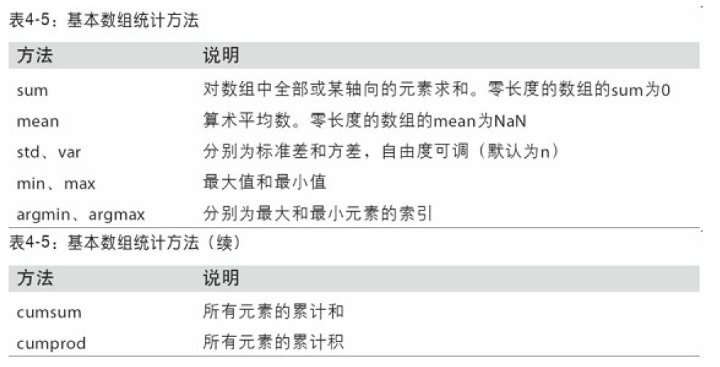
sum mean std等聚合计算
例如:随机生成一些符合正态分布的数据,然后进行聚类统计
data = np.random.randn(5,4)
data
# 结果
array([[-0.06079722,  1.49824203, -0.80957561,  0.02303306],
       [-0.96135543, -0.99023163, -2.29943668,  0.02939615],
       [-0.85931239,  0.55478495,  0.0246531 , -1.35531409],
       [ 1.4930319 , -0.51001952, -0.47922101,  0.70338996],
       [-1.14822113,  1.38053279, -0.61358326, -0.38187168]])

data.mean()
# 结果
-0.23809378534483533
np.mean(data)
# 结果
-0.23809378534483533
data.sum()
# 结果
-4.761875706896706
np.sum(data)
# 结果
-4.761875706896706
data.mean(axis=0)  # axis = 0 表示跨行---即每一列
# 结果
array([-0.30733085,  0.38666172, -0.83543269, -0.19627332])
data.sum(axis=1)   # axis = 1 表示跨列---即每一行
# 结果
array([ 0.65090226, -4.2216276 , -1.63518844,  1.20718134, -0.76314327])
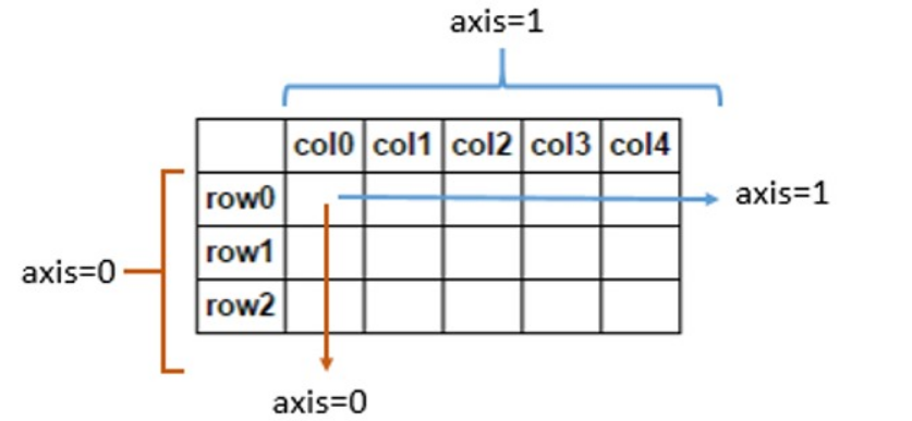
不管是mean和sum计算,最终的结果都是少一维的数组
一维的样本累加
data = np.array([1,2,3,4,5,6,7,8,9,10])
data
# array([ 1,  2,  3,  4,  5,  6,  7,  8,  9, 10])
data.cumsum()  # 功能是将样本逐渐累加
# 1 = 1;3 = 1 + 2;6 = 1 + 2 + 3;
array([ 1,  3,  6, 10, 15, 21, 28, 36, 45, 55], dtype=int32)
多维的样本累加
data = np.arange(1,10).reshape(3,3)
data
array([[1, 2, 3],
       [4, 5, 6],
       [7, 8, 9]])

data.cumsum()
# 结果
array([ 1,  3,  6, 10, 15, 21, 28, 36, 45], dtype=int32)  # 全部累加

data.cumsum(axis=0)  # 每列累加
# 结果
array([[ 1,  2,  3],
       [ 5,  7,  9],
       [12, 15, 18]], dtype=int32)

data.cumsum(axis=1)  # 每行累加
# 结果
array([[ 1,  3,  6],
       [ 4,  9, 15],
       [ 7, 15, 24]], dtype=int32)
用于布尔型的数组方法
# TODO
数组排序
sort
一维数组排序
data = np.random.randn(5)
data
# 结果
array([-2.5325336 , -0.45898654, -0.35112763, -0.93824495, -0.6494557 ])
data.sort()
data
# 结果
array([-2.5325336 , -0.93824495, -0.6494557 , -0.45898654, -0.35112763])
2019-09-23-19:37:54
多维数组排序:sort
data = np.random.randn(5,3)
data
array([[-1.09656539, -1.44675032, -0.49202197],
       [ 0.37282188, -0.24748695,  0.02384063],
       [ 0.46740851,  1.10011835,  0.47564148],
       [ 0.57882475, -2.20542035,  0.17290702],
       [ 0.55513993, -0.35427358, -2.03757406]])
data.sort(0)
data
array([[-1.09656539, -2.20542035, -2.03757406],
       [ 0.37282188, -1.44675032, -0.49202197],
       [ 0.46740851, -0.35427358,  0.02384063],
       [ 0.55513993, -0.24748695,  0.17290702],
       [ 0.57882475,  1.10011835,  0.47564148]])
np.sort(data,axis=0)
data
array([[-1.09656539, -2.20542035, -2.03757406],
       [ 0.37282188, -1.44675032, -0.49202197],
       [ 0.46740851, -0.35427358,  0.02384063],
       [ 0.55513993, -0.24748695,  0.17290702],
       [ 0.57882475,  1.10011835,  0.47564148]])
axis = 1排序结果:
array([[ 0.16578703,  0.07492019, -0.97846794],
       [-0.18209471, -0.41217471, -0.60299124],
       [-1.72009426, -0.44879286, -1.6406782 ],
       [ 1.7511948 , -0.20265756,  0.82688453],
       [-0.47502325, -0.52784722, -1.52997592]])

np.sort(data,axis=1)
array([[-0.97846794,  0.07492019,  0.16578703],
       [-0.60299124, -0.41217471, -0.18209471],
       [-1.72009426, -1.6406782 , -0.44879286],
       [-0.20265756,  0.82688453,  1.7511948 ],
       [-1.52997592, -0.52784722, -0.47502325]])
# 数组进行排序后就已经更改了数组的结构,数组变成了排序好的结构
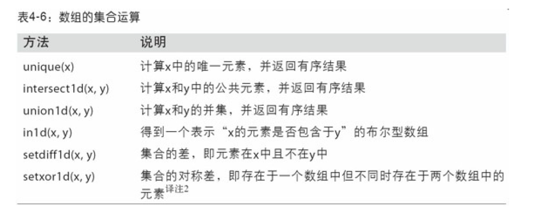
一维数组的唯一值查找方法:也可理解为去重
data = np.array([1,2,3,4,5,4,3,2,1,0])
data
array([1, 2, 3, 4, 5, 4, 3, 2, 1, 0])
np.unique(data) # 去重后并返回排序好的数组
array([0, 1, 2, 3, 4, 5])
成员是否在数组里面的判断方法
data = np.array([1,2,3,4,5,4,3,2,1,0])
data
array([1, 2, 3, 4, 5, 4, 3, 2, 1, 0])
ret = np.in1d(data,[3,4,5])
ret # 返回一个bool值的列表
array([False, False, False, False, False,  True,  True,  True,  True,
        True])
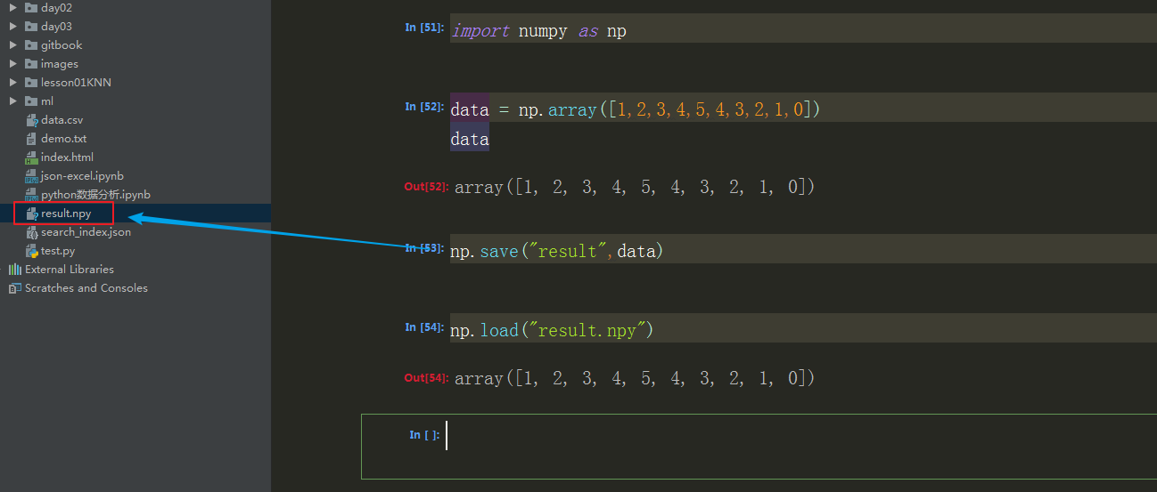
数组文件的输入和输出
numpy可以读取磁盘上的文本和二进制数据。np.save,np.load两个函数,默认下,数组是以未压缩的原始二进制格式保存在.npy的文件中。
a = np.array([1,2,3])
b = np.array([4,5,6])
c = np.array([7,8,9])

np.savez("many",a=a,b=b,c=c)  # 关键字参数传递参数

ret = np.load("many.npz")
# ret类似一个字典形式
ret
<numpy.lib.npyio.NpzFile at 0x5dda080>
ret['a']
array([1, 2, 3])
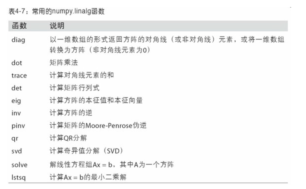
线性代数
numpy提供了dot函数,用来让两个矩阵进行乘法,
x = np.array([[1,2,3],[4,5,6]])
y = np.array([[7,8],[9,10],[11,12]])

# 2*3  3 *2 ---- 2 * 2

ret = np.dot(x,y)
ret

array([[ 58,  64],
       [139, 154]])
二维矩阵 * 一维矩阵(大小合适)
x = np.array([[1,2,3],[4,5,6]])
y = np.array([7,8,9])

y
y.shape    # 一维数组只有行,没有列

# 结果
(3,)  3 * 1

ret = np.dot(x,y) 2*3  * 3*1 = 2*1
ret
# 结果

array([ 50, 122])
矩阵的转置,矩阵的逆
data = np.random.randn(5,5)
data
array([[-0.66722861, -1.05166739,  0.50078389,  0.12101523, -1.79648742],
       [ 1.39744908,  0.52359195, -1.72793681,  0.85379089,  1.31061423],
       [-0.97876769, -0.45461206,  1.30106165,  1.24189733,  0.09226485],
       [-0.05682579, -0.86258199,  0.15000168,  0.13101571, -0.83373897],
       [-0.91637877, -0.7502237 ,  0.19909396,  0.24339183,  1.89803093]])
from numpy.linalg import inv,qr
data_r = inv(data) # 矩阵的逆矩阵
data_r
array([[-1.76904786, -0.2303984 ,  0.17920536,  2.35016865, -0.49167585],
       [ 0.4604562 ,  0.06423869,  0.12409186, -1.50670415, -0.27641049],
       [-1.5185419 , -0.58246668,  0.4536423 ,  1.57608382, -0.36483338],
       [ 0.40719248,  0.45835402,  0.51499641, -0.38190467, -0.12388313],
       [-0.56503165, -0.0835249 ,  0.02194552,  0.42277667,  0.2343783 ]])
np.dot(data,data_r)
array([[ 1.00000000e+00,  6.43952042e-17,  6.35430438e-17,
        -2.23554197e-16, -8.50732362e-17],
       [ 4.93729662e-18,  1.00000000e+00, -5.08010725e-18,
         3.01746183e-16,  1.16513398e-16],
       [-3.28852246e-16,  1.57394623e-16,  1.00000000e+00,
         2.13695858e-17, -6.72574187e-17],
       [-3.73875165e-17,  2.04305881e-17, -1.55255260e-17,
         1.00000000e+00,  8.39231877e-18],
       [-4.56471514e-17,  1.45263310e-16, -1.80718066e-18,
        -1.44115115e-16,  1.00000000e+00]])
伪随机数的生成
标准正太分布的数据样本
# TODO

 浙公网安备 33010602011771号