tensorflow之曲线拟合
视频链接:https://morvanzhou.github.io/tutorials/machine-learning/ML-intro/
1.定义层
定义 add_layer()
from __future__ import print_function
import tensorflow as tf

def add_layer(inputs, in_size, out_size, activation_function=None):
    Weights = tf.Variable(tf.random_normal([in_size, out_size]))
    biases = tf.Variable(tf.zeros([1, out_size]) + 0.1)
    Wx_plus_b = tf.matmul(inputs, Weights) + biases
    if activation_function is None:
        outputs = Wx_plus_b
    else:
        outputs = activation_function(Wx_plus_b)
    return outputs
解释
add_layer函数有四个形参。分别是
-
intputs 代表输入值,是这个神经元网络接收的数据,比如第二层网络的inputs就是第一层网络的outputs
-
in_size 代表输入的数据有几个特征,比如给苹果分类的话,特征可能有 大小、颜色、品种...
-
out_size 代表输出几个特征
-
activation_function 默认为None,即 f(x) = x
2.建造神经网络
建造神经网络代码
from __future__ import print_function
import tensorflow as tf
import numpy as np

def add_layer(inputs, in_size, out_size, activation_function=None):
    # add one more layer and return the output of this layer
    Weights = tf.Variable(tf.random_normal([in_size, out_size]))
    biases = tf.Variable(tf.zeros([1, out_size]) + 0.1)
    Wx_plus_b = tf.matmul(inputs, Weights) + biases
    if activation_function is None:
        outputs = Wx_plus_b
    else:
        outputs = activation_function(Wx_plus_b)
    return outputs

# Make up some real data
x_data = np.linspace(-1,1,300)[:, np.newaxis]
noise = np.random.normal(0, 0.05, x_data.shape)
y_data = np.square(x_data) - 0.5 + noise

# define placeholder for inputs to network
xs = tf.placeholder(tf.float32, [None, 1])
ys = tf.placeholder(tf.float32, [None, 1])
# add hidden layer
l1 = add_layer(xs, 1, 10, activation_function=tf.nn.relu)
# add output layer
prediction = add_layer(l1, 10, 1, activation_function=None)

# the error between prediction and real data
loss = tf.reduce_mean(tf.reduce_sum(tf.square(ys - prediction),
                     reduction_indices=[1]))
train_step = tf.train.GradientDescentOptimizer(0.1).minimize(loss)

# important step
# tf.initialize_all_variables() no long valid from
# 2017-03-02 if using tensorflow >= 0.12
if int((tf.__version__).split('.')[1]) < 12:
    init = tf.initialize_all_variables()
else:
    init = tf.global_variables_initializer()
sess = tf.Session()
sess.run(init)

for i in range(1000):
    # training
    sess.run(train_step, feed_dict={xs: x_data, ys: y_data})
    if i % 50 == 0:
        # to see the step improvement
        print(sess.run(loss, feed_dict={xs: x_data, ys: y_data}))
解释
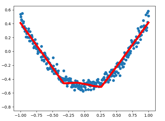
1. y_data = np.square(x_data) - 0.5 + noise ,可以看到样本数据是个二次函数
2. l1 = add_layer(xs, 1, 10, activation_function=tf.nn.relu)
① 这里添加了一个神经网络层,这一层为隐藏层(实际上这个工程一共三层),输入数据为xs ,xs 为 若干行,一列,代表这里有若干个样本数据,每个样本数据提供一个特征
所以这里in_size 为 1
② 输出10个特征,这个数值是自己添加的(你想写成12也可以,不过要和后边的代码吻合),所以这里out_size 为 10
③ 第四个参数为激励函数 , 激励函数的作用可以打开在这里看一下:https://blog.csdn.net/tyhj_sf/article/details/79932893
文中最后也说 “这个问题目前没有确定的方法,凭一些经验吧。” [无奈脸] 这里使用的relu 函数
④ 这个函数返回这若干个样本的10 个特征,赋值给l1,l1扔给后面的函数
3. prediction = add_layer(l1, 10, 1, activation_function=None) ,这就是那个后面的函数,也是添加层,这一层为输出层。
① l1是前面函数传递过来的,作为本函数的输入数据
② 这里的10 也是前边函数输出的10 个特征,这里作为输入
③ 这里的1 表示最总输出数据的列数,输入层当时提供的每个样本数据特征值为1个,作为预测,输出多个特征是不合理的/莫名其妙的,所以这里的1取决于输入样本值的特征。
④ 激励函数为None,即f(x) = x
这段代码其他地方没什么好说的
3.结果可视化
安装
matplotlib,tkinter.sudo pip3 install matplotlib sudo apt-get install pyhon-tk
代码全文
from __future__ import print_function
import tensorflow as tf
import numpy as np
import matplotlib.pyplot as plt

def add_layer(inputs, in_size, out_size, activation_function=None):
    Weights = tf.Variable(tf.random_normal([in_size, out_size]))
    biases = tf.Variable(tf.zeros([1, out_size]) + 0.1)
    Wx_plus_b = tf.matmul(inputs, Weights) + biases
    if activation_function is None:
        outputs = Wx_plus_b
    else:
        outputs = activation_function(Wx_plus_b)
    return outputs

# Make up some real data
x_data = np.linspace(-1, 1, 300)[:, np.newaxis]
noise = np.random.normal(0, 0.05, x_data.shape)
y_data = np.square(x_data) - 0.5 + noise

##plt.scatter(x_data, y_data)
##plt.show()

# define placeholder for inputs to network
xs = tf.placeholder(tf.float32, [None, 1])
ys = tf.placeholder(tf.float32, [None, 1])
# add hidden layer
l1 = add_layer(xs, 1, 10, activation_function=tf.nn.relu)
# add output layer
prediction = add_layer(l1, 10, 1, activation_function=None)

# the error between prediction and real data
loss = tf.reduce_mean(tf.reduce_sum(tf.square(ys-prediction), reduction_indices=[1]))
train_step = tf.train.GradientDescentOptimizer(0.1).minimize(loss)
# important step
sess = tf.Session()
# tf.initialize_all_variables() no long valid from
# 2017-03-02 if using tensorflow >= 0.12
if int((tf.__version__).split('.')[1]) < 12 and int((tf.__version__).split('.')[0]) < 1:
    init = tf.initialize_all_variables()
else:
    init = tf.global_variables_initializer()
sess.run(init)

# plot the real data
fig = plt.figure()
ax = fig.add_subplot(1,1,1)
ax.scatter(x_data, y_data)
plt.ion()
plt.show()


for i in range(1000):
    # training
    sess.run(train_step, feed_dict={xs: x_data, ys: y_data})
    if i % 50 == 0:
        # to visualize the result and improvement
        try:
            ax.lines.remove(lines[0])
        except Exception:
            pass
        prediction_value = sess.run(prediction, feed_dict={xs: x_data})
        # plot the prediction
        lines = ax.plot(x_data, prediction_value, 'r-', lw=5)
        plt.pause(1)
拟合曲线展示
解释
-
程序中有两次作图,一次是散点的展示,用的函数是
ax.scatter(x_data, y_data),另一次是画出拟合的曲线ax.plot(x_data, prediction_value,),注意,这两个函数分别对应 点 和 线 。 -
ax.lines.remove(lines[0]) ,你和图像的过程是逐渐向正确方向靠拢的过程,所以拟合的曲线也是动态变化的,新的曲线绘制出来的前一瞬间,需要把上一次绘制的拟合曲线删除,就是这句代买的作用
-
prediction_value = sess.run(prediction, feed_dict={xs: x_data}) 获取本次最新训练的预测结果
-
lines = ax.plot(x_data, prediction_value, 'r-', lw=5) , 将样本数据x,预测结果进行拟合,得到曲线图
-
plt.pause(1) ,图像暂停1s ,以供程序员观察图像
总结
神奇的激励函数
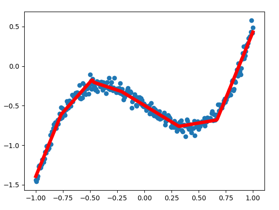
我用这套代码拟合曲线 y_data = 2*x_data*np.square(x_data) - x_data - 0.5 + noise ,发现拟合的也不错,两个样本差别不小的。上边的图像为U行,这里为N形。如下图。
思考
这套代码差不多是我最初接触到的完整代码,但是随着看其他教程推演,第三次看这套代码才看明白。
不能说全明白,比如
- 问题1: 什么情况下使用什么样的激励函数 这个问题,就没有答案。
- 问题2:在这个demo中怎么叫训练好的模型。整个拟合过程也没有可以输出的中间参数
这个问题已经解决了
训练好的模型,就是输出中间权重参数(Weights),和偏差参数(biases)
基本原理:上面提供的代码神经网络共三层,输入层,隐藏层,输出层,其中隐藏层和输出层使用了add_layer()函数,也就是这两层有各自的权重参数和偏差参数。因为这两层的输入(in_size)和输出(out_size)不同,所以这两层的参数的行列数(shape)也是相应不同的。
接下来我们把训练好的参数取出来
① 添加全局变量。在add_layer 函数前边添加
Weights = tf.Variable([-1,-1],dtype = tf.float32)
biases = tf.Variable([-1,-1],dtype = tf.float32)
Weights2 = tf.Variable([-1,-1],dtype = tf.float32)
biases2 = tf.Variable([-1,-1],dtype = tf.float32)
② 改返回,把
return outputs
改为
return outputs,Weights,biases
③ 改接收,把
l1 = add_layer(xs, 1, 10, activation_function=tf.nn.relu)
prediction = add_layer(l1, 10, 1, activation_function=None)
改为
l1,Weights,biases = add_layer(xs, 1, 10, activation_function=tf.nn.relu)
prediction,Weights2,biases2 = add_layer(l1, 10, 1, activation_function=None)
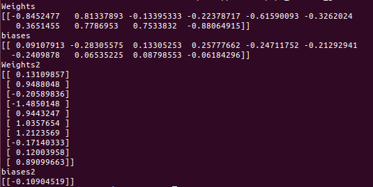
④ 在最后添加代码打印这些参数
print("Weights")
print(Weights)
print("biases")
print(biases)
print("Weights2")
print(Weights2)
print("biases2")
print(biases2)
打印参数结果
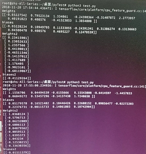
- 问题3:新的结果产生新的问题。在解决问题2之后,运行代码可以得到解,但是带有隐藏层和激励函数的代码每次循行之后得到的结果不同。如以上代码,去掉noise,连续运行两次,得到的是差别比较大的两组解。
之后就什么心得体会或者思考的话再想着回来补充吧 😀

 浙公网安备 33010602011771号