
卷积神经网络基础-Pytorch
PyTorch 神经网络基础
一个最简单的神经网络定义
import torch
import torch.nn as nn

class QNetwork(nn.Module):
    def __init__(self, state_dim, action_dim, hidden_dim=128):
        super(QNetwork, self).__init__()
        self.net = nn.Sequential(
            nn.Linear(state_dim, hidden_dim),  # 第1层:输入→隐藏层
            nn.ReLU(),                          # 激活函数(非线性)
            nn.Linear(hidden_dim, hidden_dim), # 第2层:隐藏层→隐藏层
            nn.ReLU(),
            nn.Linear(hidden_dim, action_dim)  # 第3层:隐藏层→输出
        )

    def forward(self, x):
        return self.net(x)
import os                     # 导入顶级模块
import os.path as path        # 导入子模块并起别名(为了省去 os.path 的写法)
import torch
import torch.nn as nn
1. 类定义与继承
class QNetwork(nn.Module):
- 继承自
torch.nn.Module,这是 PyTorch 中所有神经网络模块的基类 - 通过继承,该网络能够自动管理参数、支持 GPU 迁移、实现训练/评估模式切换等
2. __init__ 方法
def __init__(self, state_dim, action_dim, hidden_dim=128):
参数
state_dim:状态空间的维度(输入特征数)。例如,如果状态是 4 个连续变量(CartPole 环境),则state_dim=4action_dim:动作空间的维度(输出节点数)。对于离散动作,每个动作对应一个输出 Q 值hidden_dim:隐藏层的神经元数量,默认 128
网络结构
self.net = nn.Sequential(
    nn.Linear(state_dim, hidden_dim),  # 第1层:输入 → 隐藏层
    nn.ReLU(),                          # 激活函数(增加非线性)
    nn.Linear(hidden_dim, hidden_dim), # 第2层:隐藏层 → 隐藏层
    nn.ReLU(),
    nn.Linear(hidden_dim, action_dim)  # 第3层:隐藏层 → 输出层
)
- 使用
nn.Sequential将多个层按顺序组合,方便前向传播 - 三层全连接网络(输入层不算在内):
- 输入 → 第一隐藏层(
state_dim → hidden_dim)+ ReLU - 第二隐藏层(
hidden_dim → hidden_dim)+ ReLU - 输出层(
hidden_dim → action_dim):无激活函数,因为 Q 值可以是任意实数
- 输入 → 第一隐藏层(
- 激活函数 ReLU 引入非线性,使网络能够拟合复杂的函数关系
3. forward 方法
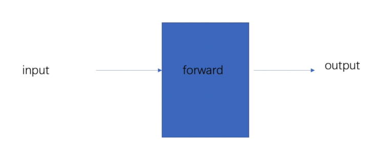
在 PyTorch 中,当你调用网络实例(例如 q_net(state))时,会自动执行 forward 函数。它是网络的核心计算逻辑。
def forward(self, x):
    return self.net(x)
- 定义输入
x如何通过网络得到输出 - 这里直接调用
self.net(x),因为nn.Sequential已经包含了所有层 x通常是状态张量,形状一般为(batch_size, state_dim),输出形状为(batch_size, action_dim),即每个动作对应的 Q 值
卷积神经网络
全连接层
nn.Linear(in_features, out_features, bias=True)
in_features:输入特征数out_features:输出特征数bias:是否使用偏置(默认 True)
layer = nn.Linear(128, 64) # 输入128维,输出64维
卷积层
步长为1,padding=0情况下:
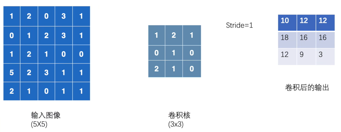
具体的PyTorch实现:
import torch
import torch.nn.functional as F

input = torch.tensor([[1, 2, 0, 3, 1],
                      [0, 1, 2, 3, 1],
                      [1, 2, 1, 0, 0],
                      [5, 2, 3, 1, 1],
                      [2, 1, 0, 1, 1]])
kernel = torch.tensor([[1, 2, 1],
                       [0, 1, 0],
                       [2, 1, 0]])

input = torch.reshape(input, [1, 1, 5, 5])
kernel = torch.reshape(kernel, [1, 1, 3, 3])

output = F.conv2d(input, kernel, stride=1, padding=0)
output = torch.reshape(output, [3, 3])
print(output)
具体文档:torch.nn.functional.conv2d — PyTorch 2.12 documentation
class torch.nn.Conv2d(in_channels, out_channels, kernel_size, stride=1, padding=0, dilation=1, groups=1, bias=True, padding_mode='zeros', device=None, dtype=None)
怎么理解卷积核的输出shape的计算公式
$$H_{\text{out}} = \left\lfloor
\frac{
H_{\text{in}}
+ 2 \times \text{padding}[0]
- \text{dilation}[0] \times (\text{kernel_size}[0] - 1)
- 1
}{
\text{stride}[0]
} + 1
\right\rfloor$$
滑了多少步?
输入宽度 W_in
卷积核宽度 kernel_size
每一步"吃掉" kernel_size 个格子
步与步之间间隔 stride
滑的步数 = (W_in - kernel_size) / stride
但这只是起始位置的数量,卷积核还要覆盖自身的宽度,所以输出宽度 = 步数 + 1(最后一个位置还能放一个卷积核):
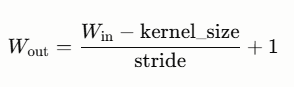
可能不是整除stride,所以向下取整。
最大池化
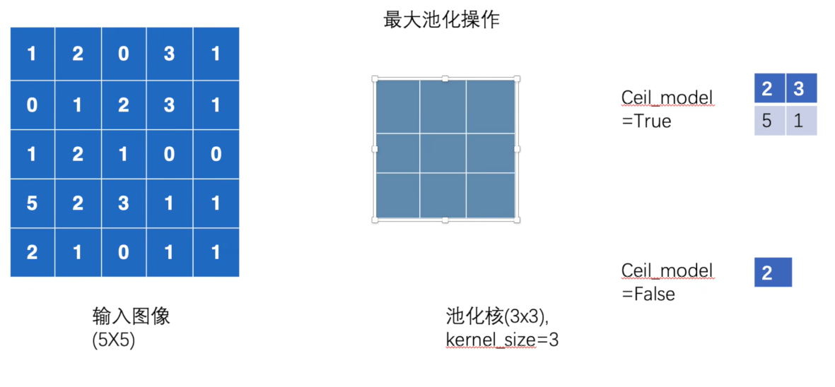
class torch.nn.MaxPool2d(kernel_size, stride=None, padding=0, dilation=1, return_indices=False, ceil_mode=False)
Parameters:
- kernel_size (int | tuple[int, int]) – the size of the window to take a max over
- stride (int | tuple[int, int]) – the stride of the window. Default value is
kernel_size - padding (int | tuple[int, int]) – Implicit negative infinity padding to be added on both sides
- dilation (int | tuple[int, int]) – a parameter that controls the stride of elements in the window
- return_indices (bool) – if
True, will return the max indices along with the outputs. Useful fortorch.nn.MaxUnpool2dlater - ceil_mode (bool) – when True, will use ceil instead of floor to compute the output shape
ceil_mode操作演示
# 最大池化
import torch
import torch.nn as nn

input = torch.tensor([[1, 2, 0, 3, 1],
                      [0, 1, 2, 3, 1],
                      [1, 2, 1, 0, 0],
                      [5, 2, 3, 1, 1],
                      [2, 1, 0, 1, 1]])

class MyNet(nn.Module):
    def __init__(self):
        super(MyNet, self).__init__()
        self.maxPool1 = nn.MaxPool2d(kernel_size=3, ceil_mode=True)

    def forward(self, x):
        x = self.maxPool1(x)
        return x

input = torch.reshape(input, [1, 1, 5, 5])
mynet = MyNet()
output = mynet(input)
print(output)
注意:(N, C, H, W) — nn.MaxPool2d 要求的输入格式是 4维
| 维度 | 含义 |
|---|---|
| N | 批次 |
| C | 通道 |
| H | 高 |
| W | 宽 |
激活函数
激活函数为神经网络引入非线性,使其能够学习和表示复杂的函数映射。
常见的激活函数:ReLU、Sigmoid、Softmax 等
现代网络 90% 的情况用 ReLU 或 GELU,其他激活函数主要出现在特定场景。
m = nn.ReLU()
input = torch.randn(2)
output = m(input)
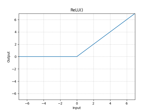
ReLU
- 输出范围:[0, +∞)
- 优点:计算极快(一个 if 判断)、缓解梯度消失(正区间梯度恒为 1)
- 缺点:Dying ReLU — 负区间永远输出 0,梯度为 0,某些神经元可能"死掉"
- 用途:几乎所有现代网络默认首选
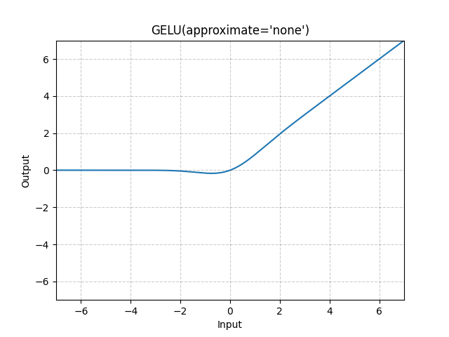
GELU
特点:比 ReLU 更平滑,Transformer(BERT、GPT)都用它
| 场景 | 推荐 |
|---|---|
| 隐藏层(通用) | ReLU |
| Transformer 类模型 | GELU |
| 二分类输出 | Sigmoid |
| 多分类输出 | Softmax |
| 怕 ReLU 死掉 | LeakyReLU |
线性层
线性层(Linear Layer)也叫全连接层(Fully Connected Layer)或仿射层(Affine Layer),是神经网络最基本的组成单元。
class torch.nn.Linear(in_features, out_features, bias=True, device=None, dtype=None)
参数:
- in_features(整数)——每个输入样本的大小
- out_features(整数)——每个输出样本的大小
- bias(布尔值)– 如果设置为
False,则该层将不会学习加性偏置。默认值:True
m = nn.Linear(20, 30)
input = torch.randn(12, 12, 20)
output = m(input)
print(output.size())
注意: nn.Linear 总是作用于输入张量的最后一个维度。
无论输入是几维张量,nn.Linear(in, out) 只关心最后一维,其他维度全部透传(batch、seq_len 等都不会受影响)。
通常作为神经网络的尾部作为分类头:
self.classifier = nn.Sequential(
    nn.Linear(512, 256),
    nn.ReLU(),
    nn.Dropout(0.5),
    nn.Linear(256, 10)    # 10分类
)
Dropout层
Dropout 是一种防止过拟合的正则化技术,通过在训练时随机"丢弃"部分神经元来工作。
具体做法
在训练过程中,以概率 p 随机地将输入张量的某些元素置零。对于每个前向调用,零元素都是独立选择的,并且是从伯努利分布中采样的。每次前向调用时,每个通道都会独立地被清零。
class MyNet(nn.Module):
    def __init__(self):
        super().__init__()
        self.fc1 = nn.Linear(512, 256)
        self.dropout = nn.Dropout(p=0.5)    # p=0.5,丢弃50%

    def forward(self, x):
        x = self.fc1(x)
        x = self.relu(x)
        x = self.dropout(x)                  # 训练时有效果,测试时自动关闭
        return x
训练 vs 测试 的区别
| 阶段 | 行为 |
|---|---|
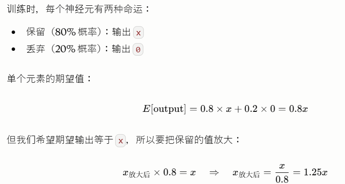
| 训练 | 以概率 p 随机丢弃神经元,剩余的输出放大 1/(1-p) |
| 测试 | 所有神经元都参与,不丢弃,但输出保持原样 |
为什么要放大?
因为训练时只有 (1-p) 的神经元在工作,期望输出变小了,测试时所有神经元都工作,所以要补偿回去。
为什么能防止过拟合?
强迫网络不依赖特定神经元。
没有 Dropout 时,网络可能学到"第 5 个神经元总是负责识别猫"——这叫协同适应(co-adaptation),某个神经元坏了网络就废了。
加 Dropout 后,第 5 个神经元可能被随机丢弃,网络被迫让多个神经元共同承担识别猫的任务,结果是泛化能力更强。
用在哪里
class FullNet(nn.Module):
    def __init__(self):
        super().__init__()
        self.net = nn.Sequential(
            nn.Linear(784, 512),
            nn.ReLU(),
            nn.Dropout(0.3),       # 第1层后

            nn.Linear(512, 256),
            nn.ReLU(),
            nn.Dropout(0.3),       # 第2层后

            nn.Linear(256, 10)
            # 输出层一般不加 Dropout
        )
通常加在隐藏层后面,不加在输出层。
| 场景 | 是否用 Dropout |
|---|---|
| 数据量小,容易过拟合 | ✅ 用 |
| 网络很深很宽 | ✅ 用 |
| 使用 L2 正则化 | 可以不用 |
| 数据量很大,训练充足 | ❌ 不需要 |
| 使用 BatchNorm | 效果重叠,可能少用 |
现代实践中,BatchNorm 和 Dropout 有时会冲突,两者同时用效果可能反而变差,所以要根据自己的网络结构调一调。
损失函数
前向传播:计算损失,即实际输出与目标输出之间的差距
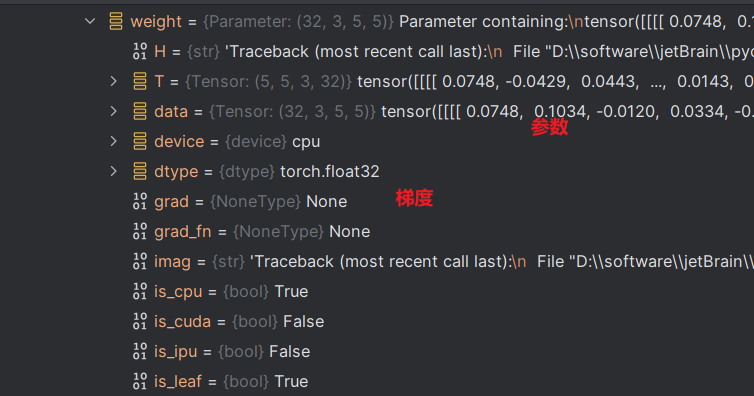
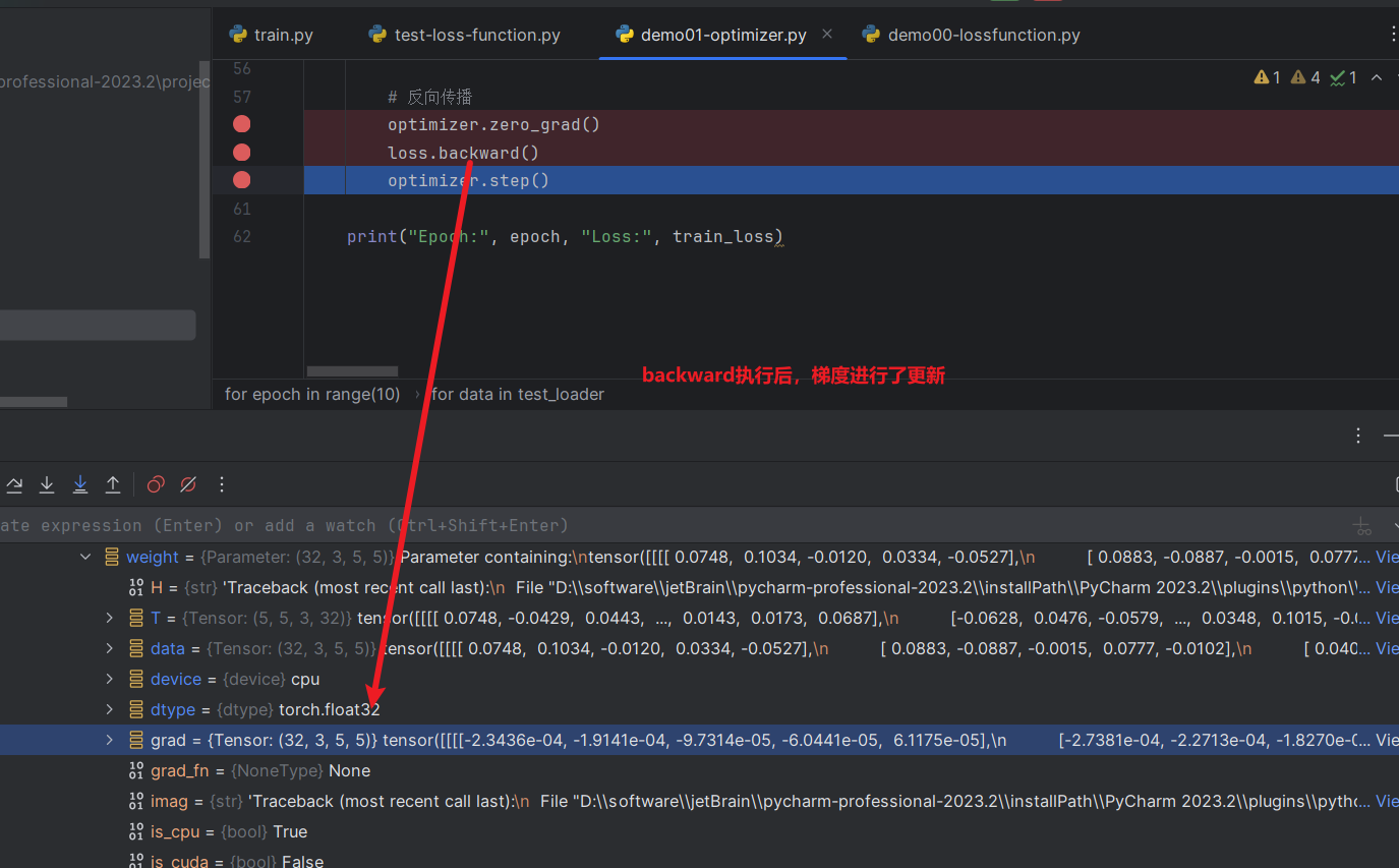
反向传播:为参数权重更新提供依据,梯度grad更新
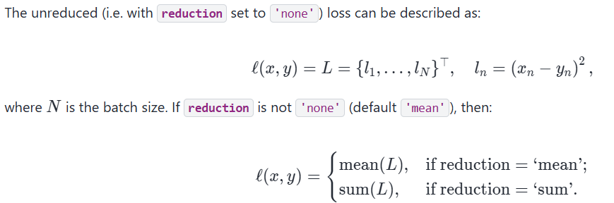
MSE损失
class torch.nn.MSELoss(size_average=None, reduce=None, reduction='mean')
import torch
from torch.nn import MSELoss

output = torch.tensor([1, 2, 3], dtype=torch.float32)
target = torch.tensor([1, 2, 5], dtype=torch.float32)
loss_fn = MSELoss(reduction='sum')  # 两种模式:mean和sum
loss = loss_fn(output, target)      # 可以断点调试这一步后grad更新

print(loss)
交叉熵损失函数
class torch.nn.CrossEntropyLoss(weight=None, size_average=None, ignore_index=-100, reduce=None, reduction='mean', label_smoothing=0.0)
import torch
from torch import optim
from torch.nn import Sequential, Conv2d, MaxPool2d, Flatten, Linear, Module, ReLU, CrossEntropyLoss
import torchvision
from torchvision.transforms import transforms

transform = transforms.Compose([
    transforms.ToTensor(),                          # 转为 Tensor,且像素值从[0,255]变成[0,1]
    transforms.Normalize((0.5, 0.5, 0.5),           # 标准化:(值 - 0.5) / 0.5
                         (0.5, 0.5, 0.5))
])
test_data = torchvision.datasets.CIFAR10(
    root='../data',           # 数据存到当前目录的 data 文件夹下
    train=False,              # 训练集(50000 张图片)
    transform=transform,      # 应用预处理
    download=True             # 没有就自动下载
)

test_loader = torch.utils.data.DataLoader(test_data, batch_size=64, shuffle=False)

class MaoNet(Module):
    def __init__(self):
        super(MaoNet, self).__init__()
        self.model1 = Sequential(
            Conv2d(3, 32, 5, padding=2),
            ReLU(),  # 激活函数
            MaxPool2d(2),
            Conv2d(32, 32, 5, padding=2),
            ReLU(),
            MaxPool2d(2),
            Conv2d(32, 64, 5, padding=2),
            ReLU(),
            MaxPool2d(2),
            Flatten(),
            Linear(1024, 64),
            ReLU(),
            Linear(64, 10)
        )

    def forward(self, x):
        x = self.model1(x)
        return x

maonet = MaoNet()
loss_fn = CrossEntropyLoss()

for data in test_loader:
    img, label = data
    output = maonet(img)
    loss = loss_fn(output, label)
    print(loss)  # 打印损失
优化器
在深度学习和机器学习中,优化器(Optimizer) 是用于更新模型参数(如权重和偏置)以最小化损失函数的算法。
torch.optim 是一个实现了多种优化算法的软件包。
optimizer = optim.SGD(model.parameters(), lr=0.01, momentum=0.9)
optimizer = optim.Adam([var1, var2], lr=0.0001)
用于计算梯度之后,调用 optimizer.step(),进行参数更新。
通常是这样:
for input, target in dataset:
    optimizer.zero_grad()        # 1. 梯度重置为0
    output = model(input)
    loss = loss_fn(output, target)
    loss.backward()              # 2. 梯度更新
    optimizer.step()             # 3. 根据梯度更新参数
网络架构搭建
CIFAR10 Net
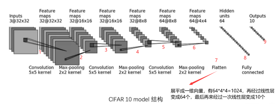
import torch
from torch.nn import Sequential, Conv2d, MaxPool2d, Flatten, Linear, Module, ReLU

class MaoNet(Module):
    def __init__(self):
        super(MaoNet, self).__init__()
        self.model1 = Sequential(
            Conv2d(3, 32, 5, padding=2),
            ReLU(),  # 激活函数
            MaxPool2d(2),
            Conv2d(32, 32, 5, padding=2),
            ReLU(),
            MaxPool2d(2),
            Conv2d(32, 64, 5, padding=2),
            ReLU(),
            MaxPool2d(2),
            Flatten(),
            Linear(1024, 64),
            ReLU(),
            Linear(64, 10)
        )

    def forward(self, x):
        x = self.model1(x)
        return x

maonet = MaoNet()
input = torch.ones([64, 3, 32, 32])
output = maonet(input)
print(output.shape)
VGG 16 Net
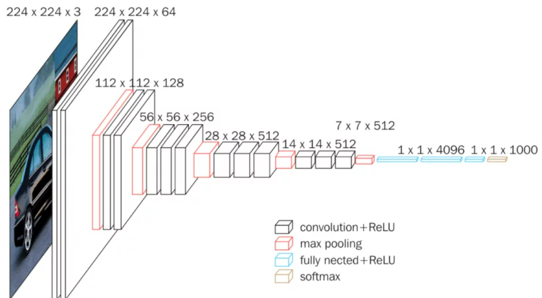
import torch
from torch.nn import Module, Sequential, Linear, ReLU, Conv2d, MaxPool2d, Softmax, Flatten

class vgg16_me(Module):
    def __init__(self):
        super(vgg16_me, self).__init__()
        self.net = Sequential(
            # Block1
            Conv2d(3, 64, 3, padding=1),
            ReLU(),
            Conv2d(64, 64, 3, padding=1),
            ReLU(),
            MaxPool2d(2),

            # Block2
            Conv2d(64, 128, 3, padding=1),
            ReLU(),
            Conv2d(128, 128, 3, padding=1),
            ReLU(),
            MaxPool2d(2),

            # Block3
            Conv2d(128, 256, 3, padding=1),
            ReLU(),
            Conv2d(256, 256, 3, padding=1),
            ReLU(),
            Conv2d(256, 256, 3, padding=1),
            ReLU(),
            MaxPool2d(2),

            # Block4
            Conv2d(256, 512, 3, padding=1),
            ReLU(),
            Conv2d(512, 512, 3, padding=1),
            ReLU(),
            Conv2d(512, 512, 3, padding=1),
            ReLU(),
            MaxPool2d(2),

            # Block5
            Conv2d(512, 512, 3, padding=1),
            ReLU(),
            Conv2d(512, 512, 3, padding=1),
            ReLU(),
            Conv2d(512, 512, 3, padding=1),
            ReLU(),
            MaxPool2d(2),
        )
        self.classify = Sequential(
            Flatten(),
            Linear(25088, 4096), ReLU(),
            Linear(4096, 4096), ReLU(),
            Linear(4096, 1000),
        )
        # 如果推理时需要 Softmax,可以手动添加
        self.softmax = Softmax(dim=1)

    def forward(self, x):
        x = self.net(x)
        x = self.classify(x)
        return x

vgg = vgg16_me()
input = torch.zeros([64, 3, 224, 224])
output = vgg(input)
print(output.shape)
ResNet 残差网络
出现原因: 网络结构越深,效果反而更差
为什么? 深度网络有梯度消失的问题
损失 → 第56层 → 第55层 → ... → 第2层 → 第1层
损失函数从后往前由复合函数求偏导的乘法法则,梯度从后往前传,每经过一层就要乘一个数。乘的数如果小于1:
0.9 × 0.9 × 0.9 × ...(乘了56次)→ 几乎为0
第一层根本收不到有效的梯度信号,学不动。
解决方法(ResNet思路): 与其让网络直接学输出,不如让它学"差值"(残差)。
- 普通网络:输出 = F(x) ← 网络要直接学 F(x)
- ResNet:输出 = x + F(x) ← 网络只需要学 F(x) = 输出 - x
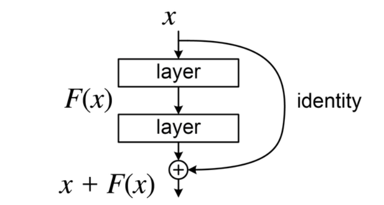
为什么学差值就简单了?
- 恒等映射对普通网络很难,对 ResNet 只需要把权重学成0
梯度怎么流?
- 普通网络:梯度 =
∂F/∂x,乘多层可能趋近于0 - ResNet:梯度 =
1 + ∂F/∂x,永远有一条"高速公路"让梯度直接流回去
import torch
from torch.nn import Module, Sequential, Linear, ReLU, Conv2d, MaxPool2d, AdaptiveAvgPool2d, Flatten

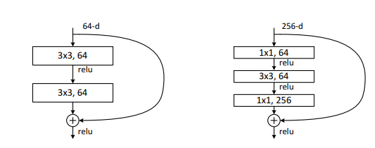
class Bottleneck(Module):
    def __init__(self, in_channels, out_channels, stride=1):
        super(Bottleneck, self).__init__()
        mid_channels = out_channels // 4

        self.core = Sequential(
            Conv2d(in_channels, mid_channels, kernel_size=1, bias=False),
            ReLU(),
            Conv2d(mid_channels, mid_channels, kernel_size=3, stride=stride, padding=1, bias=False),
            ReLU(),
            Conv2d(mid_channels, out_channels, kernel_size=1, bias=False)
        )

        # 残差连接:当输入输出维度不同时,用1x1卷积把x映射到相同维度
        self.shortcut = Sequential()
        if in_channels != out_channels:
            self.shortcut = Sequential(
                Conv2d(in_channels, out_channels, kernel_size=1, stride=stride, bias=False)
            )

        self.relu = ReLU()

    def forward(self, x):
        out = self.core(x)
        residual = self.shortcut(x)   # 维度对齐
        out = self.relu(out + residual)
        return out

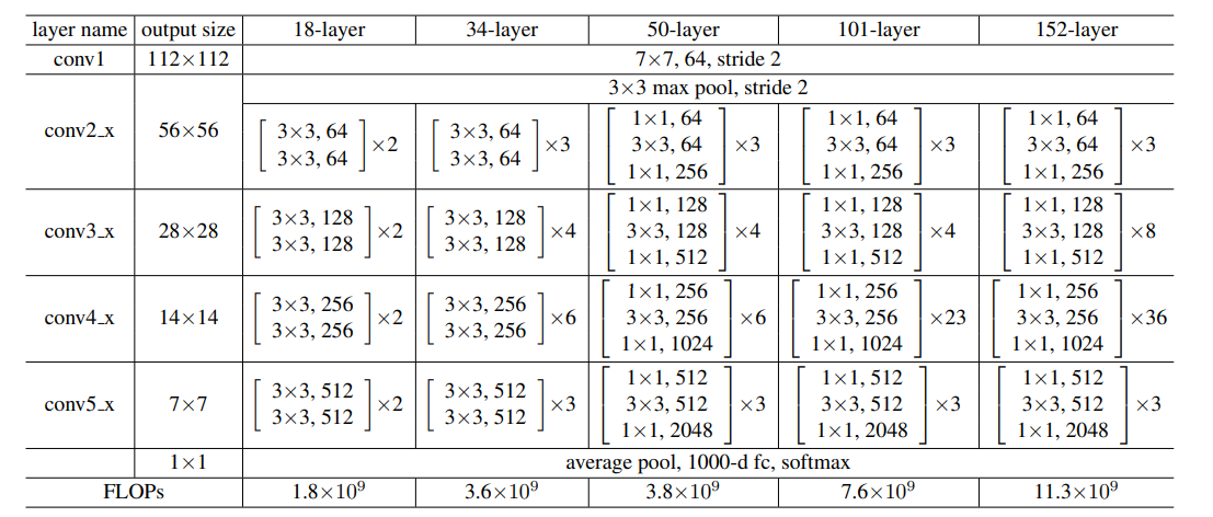
class ResNet50(Module):
    def __init__(self, num_classes=1000):
        super(ResNet50, self).__init__()

        # ── header: 224×224 → 56×56 ──
        self.header = Sequential(
            Conv2d(3, 64, kernel_size=7, stride=2, padding=3, bias=False),
            ReLU(),
            MaxPool2d(kernel_size=3, stride=2, padding=1)
        )

        # ── body: 4个stage,分别有 3, 4, 6, 3 个 Bottleneck ──
        self.stage1 = self._make_stage(64, 256, num_blocks=3, stride=1)
        self.stage2 = self._make_stage(256, 512, num_blocks=4, stride=2)
        self.stage3 = self._make_stage(512, 1024, num_blocks=6, stride=2)
        self.stage4 = self._make_stage(1024, 2048, num_blocks=3, stride=2)

        # ── tail: 全局平均池化 + 全连接 ──
        self.classify = Sequential(
            AdaptiveAvgPool2d(1),       # 2048 × 7 × 7 → 2048 × 1 × 1
            Flatten(),                  # → 2048
            Linear(2048, num_classes)    # → 1000
        )

    def _make_stage(self, in_channels, out_channels, num_blocks, stride):
        layers = []
        layers.append(Bottleneck(in_channels, out_channels, stride))
        for _ in range(1, num_blocks):
            layers.append(Bottleneck(out_channels, out_channels, stride=1))
        return Sequential(*layers)

    def forward(self, x):
        x = self.header(x)       # 224 → 56
        x = self.stage1(x)       # 56 × 56
        x = self.stage2(x)       # 28 × 28
        x = self.stage3(x)       # 14 × 14
        x = self.stage4(x)       # 7 × 7
        x = self.classify(x)     # 1000
        return x

# 测试
model = ResNet50(num_classes=1000)
input = torch.zeros([64, 3, 224, 224])
output = model(input)
print(output.shape)   # torch.Size([64, 1000])
网络模型的使用
torchvision提供一系列的视觉相关的模型和模型的预训练参数
Models and pre-trained weights — Torchvision 0.27 documentation
实例化预训练模型会将权重下载到缓存目录。可以使用 TORCH_HOME 环境变量设置此目录。
import os
from torchvision.models import vgg16

# 设置模型保存路径
os.environ['TORCH_HOME'] = '../weights'

# deprecated
# model_false = vgg16(pretrained=False)
# model_true = vgg16(pretrained=True)

model_false = vgg16(weights=None)
model_true = vgg16(weights='DEFAULT', progress=True)
print(model_true)
初始化预训练模型
加载权重文件:
# 1. 先创建空模型
model_true = vgg16(weights=None)   # 不下载,不加载预训练权重

# 2. 加载本地权重文件
model.load_state_dict(torch.load('model.pth', weights_only=True))  # .pth 文件路径
strict=False 让你只加载能对上的部分,对不上的保持随机初始化,然后用新数据微调。这就是迁移学习的核心思路。
model_state_dict = torch.load('../weights/vgg16-397923af.pth', weights_only=True)
model_true.load_state_dict(model_state_dict, strict=False)
如何修改已有的模型
以VGG16为例:
VGG(
  (features): Sequential(
    (0): Conv2d(3, 64, kernel_size=(3, 3), stride=(1, 1), padding=(1, 1))
    (1): ReLU(inplace=True)
    (2): Conv2d(64, 64, kernel_size=(3, 3), stride=(1, 1), padding=(1, 1))
    (3): ReLU(inplace=True)
    (4): MaxPool2d(kernel_size=2, stride=2, padding=0, dilation=1, ceil_mode=False)
    (5): Conv2d(64, 128, kernel_size=(3, 3), stride=(1, 1), padding=(1, 1))
    (6): ReLU(inplace=True)
    (7): Conv2d(128, 128, kernel_size=(3, 3), stride=(1, 1), padding=(1, 1))
    (8): ReLU(inplace=True)
    (9): MaxPool2d(kernel_size=2, stride=2, padding=0, dilation=1, ceil_mode=False)
    (10): Conv2d(128, 256, kernel_size=(3, 3), stride=(1, 1), padding=(1, 1))
    (11): ReLU(inplace=True)
    (12): Conv2d(256, 256, kernel_size=(3, 3), stride=(1, 1), padding=(1, 1))
    (13): ReLU(inplace=True)
    (14): Conv2d(256, 256, kernel_size=(3, 3), stride=(1, 1), padding=(1, 1))
    (15): ReLU(inplace=True)
    (16): MaxPool2d(kernel_size=2, stride=2, padding=0, dilation=1, ceil_mode=False)
    (17): Conv2d(256, 512, kernel_size=(3, 3), stride=(1, 1), padding=(1, 1))
    (18): ReLU(inplace=True)
    (19): Conv2d(512, 512, kernel_size=(3, 3), stride=(1, 1), padding=(1, 1))
    (20): ReLU(inplace=True)
    (21): Conv2d(512, 512, kernel_size=(3, 3), stride=(1, 1), padding=(1, 1))
    (22): ReLU(inplace=True)
    (23): MaxPool2d(kernel_size=2, stride=2, padding=0, dilation=1, ceil_mode=False)
    (24): Conv2d(512, 512, kernel_size=(3, 3), stride=(1, 1), padding=(1, 1))
    (25): ReLU(inplace=True)
    (26): Conv2d(512, 512, kernel_size=(3, 3), stride=(1, 1), padding=(1, 1))
    (27): ReLU(inplace=True)
    (28): Conv2d(512, 512, kernel_size=(3, 3), stride=(1, 1), padding=(1, 1))
    (29): ReLU(inplace=True)
    (30): MaxPool2d(kernel_size=2, stride=2, padding=0, dilation=1, ceil_mode=False)
  )
  (avgpool): AdaptiveAvgPool2d(output_size=(7, 7))
  (classifier): Sequential(
    (0): Linear(in_features=25088, out_features=4096, bias=True)
    (1): ReLU(inplace=True)
    (2): Dropout(p=0.5, inplace=False)
    (3): Linear(in_features=4096, out_features=4096, bias=True)
    (4): ReLU(inplace=True)
    (5): Dropout(p=0.5, inplace=False)
    (6): Linear(in_features=4096, out_features=1000, bias=True)
  )
)
尾部增加模块,使用 add_module:
model.add_module("classify head", Linear(1000, 10))

# 或者增加到分类头里面去
model.classifier.add_module("classify head", Linear(1000, 10))
修改中间层,直接使用数组下标修改:
model.classifier[6] = Linear(4096, 10)
模型保存
模型保存有两种方式:
torch.save(model, "./XXX.pth")
torch.save(model.state_dict(), "./XXX.pth")  # 官方推荐
torch.save(model, ...) |
torch.save(model.state_dict(), ...) |
|
|---|---|---|
| 保存的是什么 | 整个模型(结构 + 权重) | 只有权重参数 |
| 文件大小 | 大(包含模型类定义) | 小(只有数据) |
| 加载方式 | torch.load(path) 直接用 |
需要先建模型再填权重 |
训练部分层
方法一:冻结部分层
# 先冻结所有参数
for param in model.parameters():
    param.requires_grad = False

# 只解冻新的全连接层
for param in model.fc.parameters():
    param.requires_grad = True
方法二:直接将需要训练的层传入优化器
optimizer = torch.optim.SGD(model.fc.parameters(), lr=0.001, momentum=0.9)
# 或者用 Adam
optimizer = torch.optim.Adam(model.fc.parameters(), lr=0.001)
模型训练总流程
import torch
import torchvision
from torch.nn import CrossEntropyLoss
from torch.utils.data import DataLoader
from torchvision import transforms
from model import MaoNet

# 1. 预处理
transform = transforms.Compose([
    transforms.ToTensor(),                          # 转为 Tensor,且像素值从[0,255]变成[0,1]
    transforms.Normalize((0.5, 0.5, 0.5),           # 标准化:(值 - 0.5) / 0.5
                         (0.5, 0.5, 0.5))
])

# 2. 数据集
train_data = torchvision.datasets.CIFAR10(
    root='./data',           # 数据存到当前目录的 data 文件夹下
    train=True,              # 训练集(50000 张图片)
    transform=transform,     # 应用预处理
    download=True            # 没有就自动下载
)

test_data = torchvision.datasets.CIFAR10(
    root='./data',
    train=False,             # 测试集(10000 张图片)
    transform=transform,
    download=True
)

# 3. DataLoader:把数据分批次加载
train_loader = DataLoader(train_data, batch_size=64, shuffle=True)
test_loader  = DataLoader(test_data,  batch_size=64, shuffle=False)

# CIFAR-10 的 10 个类别
classes = ('飞机', '汽车', '鸟', '猫', '鹿', '狗', '青蛙', '马', '船', '卡车')

# ============================================================
# 4. 初始化模型、损失函数、优化器
# ============================================================
device = torch.device('cuda' if torch.cuda.is_available() else 'cpu')

maonet = MaoNet().to(device)
loss_fn = CrossEntropyLoss()                       # 分类用交叉熵损失
optimizer = torch.optim.Adam(maonet.parameters(), lr=0.001)  # Adam 优化器

# ============================================================
# 5. 训练
# ============================================================
total_train_step = 0

for epoch in range(10):  # 训练 10 轮
    maonet.train()  # 切换到训练模式(Dropout/BatchNorm 会不同)
    total_loss = 0

    for images, labels in train_loader:
        images = images.to(device)
        labels = labels.to(device)

        # 前向传播
        outputs = maonet(images)
        loss = loss_fn(outputs, labels)

        # 反向传播
        optimizer.zero_grad()  # 5.1 清空之前的梯度
        loss.backward()        # 5.2 计算梯度
        optimizer.step()       # 5.3 更新参数

        total_loss += loss.item()
        total_train_step += 1

    avg_loss = total_loss / len(train_loader)

    # ============================================================
    # 6. 每轮结束后在测试集上验证
    # ============================================================
    maonet.eval()  # 6.1 切换到测试模式
    total_correct = 0
    total_samples = 0

    with torch.no_grad():  # 6.2 测试时不需要计算梯度
        for images, labels in test_loader:
            images = images.to(device)
            labels = labels.to(device)

            outputs = maonet(images)
            _, predicted = torch.max(outputs, 1)  # 取最大值对应的类别

            total_correct += (predicted == labels).sum().item()
            total_samples += labels.size(0)

    accuracy = total_correct / total_samples * 100
    print(f"Epoch [{epoch+1}/10]  Loss: {avg_loss:.4f}  测试准确率: {accuracy:.2f}%")

print("训练完成!")
整体框架伪代码
# ============================================================
# 1. 准备数据
# ============================================================
transform = transforms.Compose([...])                              # 数据预处理
train_dataset = Dataset(root='...', train=True, transform=transform)  # 训练集
test_dataset  = Dataset(root='...', train=False, transform=transform) # 测试集
train_loader  = DataLoader(train_dataset, batch_size=64, shuffle=True)
test_loader   = DataLoader(test_dataset,  batch_size=64, shuffle=False)

# ============================================================
# 2. 定义模型
# ============================================================
class MyNet(nn.Module):
    def __init__(self):
        # 定义网络结构:Conv → ReLU → Pool → ... → FC → Output

    def forward(self, x):
        # 前向传播,定义数据怎么流过网络
        return x

# ============================================================
# 3. 初始化三件套
# ============================================================
model     = MyNet()
loss_fn   = nn.CrossEntropyLoss()                    # 损失函数
optimizer = torch.optim.Adam(model.parameters())      # 优化器

# ============================================================
# 4. 训练循环
# ============================================================
for epoch in range(N):
    model.train()                     # 切训练模式
    for images, labels in train_loader:
        outputs = model(images)        # 前向传播 → 自动建计算图
        loss = loss_fn(outputs, labels) # 算损失

        optimizer.zero_grad()          # 清梯度
        loss.backward()                # 算梯度(沿计算图反向传播)
        optimizer.step()               # 更新参数

    # ============================================================
    # 5. 测试
    # ============================================================
    model.eval()                       # 切测试模式
    with torch.no_grad():             # 不需要梯度
        for images, labels in test_loader:
            outputs = model(images)
            _, predicted = torch.max(outputs, 1)
            # 统计正确率
训练流程:
epoch 外循环
  ↓
  batch 内循环
    ↓
    前向传播 → 损失 → 清梯度 → 反向传播 → 更新参数

 浙公网安备 33010602011771号