Mnist手写数字识别 Tensorflow
Mnist手写数字识别 Tensorflow
任务目标
- 了解mnist数据集
- 搭建和测试模型
- 利用模型识别手写数字图片
编辑环境
操作系统:Win10
python版本:3.6
集成开发环境:pycharm
tensorflow版本:1.*
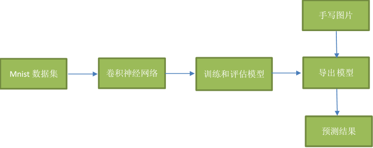
程序流程图
了解mnist数据集
mnist数据集:mnist数据集下载地址
MNIST 数据集来自美国国家标准与技术研究所, National Institute of Standards and Technology (NIST). 训练集 (training set) 由来自 250 个不同人手写的数字构成, 其中 50% 是高中学生, 50% 来自人口普查局 (the Census Bureau) 的工作人员. 测试集(test set) 也是同样比例的手写数字数据.
图片是以字节的形式进行存储, 我们需要把它们读取到 NumPy array 中, 以便训练和测试算法。
读取mnist数据集
mnist = input_data.read_data_sets("mnist_data", one_hot=True)
模型结构
输入层
with tf.variable_scope("data"):
      x = tf.placeholder(tf.float32,shape=[None,784],name='x_pred') # 784=28*28*1 宽长为28,单通道图片
      y_true = tf.placeholder(tf.int32,shape=[None,10]) # 10个类别
第一层卷积
现在我们可以开始实现第一层了。它由一个卷积接一个max pooling完成。卷积在每个5x5的patch中算出32个特征。卷积的权重张量形状是[5, 5, 1, 32],前两个维度是patch的大小,接着是输入的通道数目,最后是输出的通道数目。 而对于每一个输出通道都有一个对应的偏置量。
为了用这一层,我们把x变成一个4d向量,其第2、第3维对应图片的宽、高,最后一维代表图片的颜色通道数(因为是灰度图所以这里的通道数为1,如果是rgb彩色图,则为3)。
我们把x_image和权值向量进行卷积,加上偏置项,然后应用ReLU激活函数,最后进行max pooling。
with tf.variable_scope("conv1"):
      w_conv1 = tf.Variable(tf.random_normal([5,5,1,32])) # 5*5的卷积核  1个通道的输入图像  32个不同的卷积核,得到32个特征图
      b_conv1 = tf.Variable(tf.constant(0.0,shape=[32]))
      x_reshape = tf.reshape(x,[-1,28,28,1]) # n张 28*28 的单通道图片
      conv1 = tf.nn.relu(tf.nn.conv2d(x_reshape,w_conv1,strides=[1,1,1,1],padding="SAME")+b_conv1) #strides为过滤器步长 padding='SAME' 边缘自动补充
      pool1 = tf.nn.max_pool(conv1,ksize=[1,2,2,1],strides=[1,2,2,1],padding="SAME") # ksize为池化层过滤器的尺度,strides为过滤器步长  padding="SAME" 考虑边界,如果不够用 用0填充
第二层卷积
为了构建一个更深的网络,我们会把几个类似的层堆叠起来。第二层中,每个5x5的patch会得到64个特征
with tf.variable_scope("conv2"):
    w_conv2 = tf.Variable(tf.random_normal([5,5,32,64]))
    b_conv2 = tf.Variable(tf.constant(0.0,shape=[64]))
    conv2 = tf.nn.relu(tf.nn.conv2d(pool1,w_conv2,strides=[1,1,1,1],padding="SAME")+b_conv2)
    pool2 = tf.nn.max_pool(conv2,ksize=[1,2,2,1],strides=[1,2,2,1],padding="SAME")
密集连接层
现在,图片尺寸减小到7x7,我们加入一个有1024个神经元的全连接层,用于处理整个图片。我们把池化层输出的张量reshape成一些向量,乘上权重矩阵,加上偏置,然后对其使用ReLU。
为了减少过拟合,我们在输出层之前加入dropout。我们用一个placeholder来代表一个神经元的输出在dropout中保持不变的概率。这样我们可以在训练过程中启用dropout,在测试过程中关闭dropout。 TensorFlow的tf.nn.dropout操作除了可以屏蔽神经元的输出外,还会自动处理神经元输出值的scale。所以用dropout的时候可以不用考虑scale。
with tf.variable_scope("fc1"):
      w_fc1 = tf.Variable(tf.random_normal([7*7*64,1024])) # 经过两次卷积和池化 28 * 28/(2+2) = 7 * 7
      b_fc1 = tf.Variable(tf.constant(0.0,shape=[1024]))
      h_pool2_flat = tf.reshape(pool2, [-1, 7 * 7 * 64])
      h_fc1 = tf.nn.relu(tf.matmul(h_pool2_flat, w_fc1) + b_fc1)
      # 在输出层之前加入dropout以减少过拟合
      keep_prob = tf.placeholder("float32",name="keep_prob")
      h_fc1_drop = tf.nn.dropout(h_fc1, keep_prob)
输出层
最后,我们添加一个softmax层,就像前面的单层softmax regression一样。
with tf.variable_scope("fc2"):
      w_fc2 = tf.Variable(tf.random_normal([1024,10])) # 经过两次卷积和池化 28 * 28/(2+2) = 7 * 7
      b_fc2 = tf.Variable(tf.constant(0.0,shape=[10]))
      y_predict = tf.matmul(h_fc1_drop,w_fc2)+b_fc2
      tf.add_to_collection('pred_network', y_predict)  # 用于加载模型获取要预测的网络结构
训练和评估模型
为了进行训练和评估,我们使用与之前简单的单层SoftMax神经网络模型几乎相同的一套代码,只是我们会用更加复杂的ADAM优化器来做梯度最速下降,在feed_dict中加入额外的参数keep_prob来控制dropout比例。然后每100次迭代输出一次日志。
with tf.variable_scope("loss"):
loss = tf.reduce_mean(tf.nn.softmax_cross_entropy_with_logits(labels=y_true,logits=y_predict))
with tf.variable_scope("optimizer"):
# 使用反向传播,利用优化器使损失函数最小化
train_op = tf.train.AdamOptimizer(0.001).minimize(loss)
with tf.variable_scope("acc"):
# 检测我们的预测是否真实标签匹配(索引位置一样表示匹配)
# tf.argmax(y_conv,dimension), 返回最大数值的下标 通常和tf.equal()一起使用,计算模型准确度
# dimension=0 按列找 dimension=1 按行找
equal_list = tf.equal(tf.arg_max(y_true,1),tf.arg_max(y_predict,1))
# 统计测试准确率, 将correct_prediction的布尔值转换为浮点数来代表对、错,并取平均值。
accuracy = tf.reduce_mean(tf.cast(equal_list,tf.float32))
# tensorboard
# tf.summary.histogram用来显示直方图信息
# tf.summary.scalar用来显示标量信息
# Summary:所有需要在TensorBoard上展示的统计结果
tf.summary.histogram("weight",w_fc2)
tf.summary.histogram("bias",b_fc2)
tf.summary.scalar("loss",loss)
tf.summary.scalar("acc",accuracy)
merged = tf.summary.merge_all()
saver = tf.train.Saver()
with tf.Session() as sess:
sess.run(tf.global_variables_initializer())
filewriter = tf.summary.FileWriter("tfboard",graph=sess.graph)
if is_train: # 训练
for i in range(20001):
x_train, y_train = mnist.train.next_batch(50)
if i%100==0:
# 评估模型准确度,此阶段不使用Dropout
print("第%d训练,准确率为%f" % (i + 1, sess.run(accuracy, feed_dict={x: x_train, y_true: y_train, keep_prob: 1.0})))
# # 训练模型,此阶段使用50%的Dropout
sess.run(train_op,feed_dict={x:x_train,y_true:y_train,keep_prob: 0.5})
summary = sess.run(merged,feed_dict={x:x_train,y_true:y_train, keep_prob: 1})
filewriter.add_summary(summary,i)
saver.save(sess,savemodel)
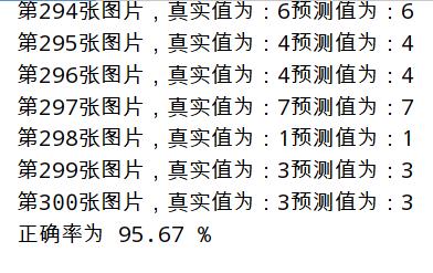
else: # 测试集预测
count = 0.0
epochs = 300
saver.restore(sess, savemodel)
for i in range(epochs):
x_test, y_test = mnist.train.next_batch(1)
print("第%d张图片,真实值为:%d预测值为:%d" % (i + 1,
tf.argmax(sess.run(y_true, feed_dict={x: x_test, y_true: y_test,keep_prob: 1.0}),
1).eval(),
tf.argmax(
sess.run(y_predict, feed_dict={x: x_test, y_true: y_test,keep_prob: 1.0}),
1).eval()
))
if (tf.argmax(sess.run(y_true, feed_dict={x: x_test, y_true: y_test,keep_prob: 1.0}), 1).eval() == tf.argmax(
sess.run(y_predict, feed_dict={x: x_test, y_true: y_test,keep_prob: 1.0}), 1).eval()):
count = count + 1
print("正确率为 %.2f " % float(count * 100 / epochs) + "%")
评估结果
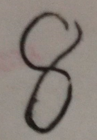
传入手写图片,利用模型预测
首先利用opencv包将图片转为单通道(灰度图),调整图像尺寸28*28,并且二值化图像,通过处理最后得到一个(0~1)扁平的图片像素值(一个二维数组)。
手写数字图片
处理手写数字图片
def dealFigureImg(imgPath):
    img = cv2.imread(imgPath)  # 手写数字图像所在位置
    img = cv2.cvtColor(img, cv2.COLOR_BGR2GRAY)  # 转换图像为单通道(灰度图)
    resize_img = cv2.resize(img, (28, 28))  # 调整图像尺寸为28*28
    ret, thresh_img = cv2.threshold(resize_img, 127, 255, cv2.THRESH_BINARY)  # 二值化
    cv2.imwrite("image/temp.jpg",thresh_img)
    im = Image.open('image/temp.jpg')
    data = list(im.getdata()) # 得到一个扁平的 图片像素
    result = [(255 - x) * 1.0 / 255.0 for x in data] # 像素值范围(0-255),转换为(0-1) ->符合模型训练时传入数据的值
    result = np.expand_dims(result, 0) # 扩展维度 ->符合模型训练时传入数据的维度
    os.remove('image/temp.jpg')
    return result
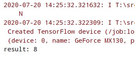
载入模型进行预测
def predictFigureImg(imgPath):
    result = dealFigureImg(imgPath)
    with tf.Session() as sess:
        new_saver = tf.train.import_meta_graph("model/mnist_model.meta")
        new_saver.restore(sess, "model/mnist_model")
        graph = tf.get_default_graph()
        x = graph.get_operation_by_name('data/x_pred').outputs[0]
        keep_prob = graph.get_operation_by_name('fc1/keep_prob').outputs[0]
        y = tf.get_collection("pred_network")[0]
        predict = np.argmax(sess.run(y, feed_dict={x: result,keep_prob:1.0}))
        print("result:",predict)
预测结果
完整代码
import tensorflow as tf
import cv2
import os
import numpy as np
from PIL import Image
from tensorflow.examples.tutorials.mnist import input_data

# 构造模型
def getMnistModel(savemodel,is_train):
    """
    :param savemodel:  模型保存路径
    :param is_train: True为训练,False为测试模型
    :return:None
    """
    mnist = input_data.read_data_sets("mnist_data", one_hot=True)
    with tf.variable_scope("data"):
        x = tf.placeholder(tf.float32,shape=[None,784],name='x_pred') # 784=28*28*1 宽长为28,单通道图片
        y_true = tf.placeholder(tf.int32,shape=[None,10]) # 10个类别

    with tf.variable_scope("conv1"):
        w_conv1 = tf.Variable(tf.random_normal([5,5,1,32])) # 5*5的卷积核  1个通道的输入图像  32个不同的卷积核,得到32个特征图
        b_conv1 = tf.Variable(tf.constant(0.0,shape=[32]))
        x_reshape = tf.reshape(x,[-1,28,28,1]) # n张 28*28 的单通道图片
        conv1 = tf.nn.relu(tf.nn.conv2d(x_reshape,w_conv1,strides=[1,1,1,1],padding="SAME")+b_conv1) #strides为过滤器步长 padding='SAME' 边缘自动补充
        pool1 = tf.nn.max_pool(conv1,ksize=[1,2,2,1],strides=[1,2,2,1],padding="SAME") # ksize为池化层过滤器的尺度,strides为过滤器步长  padding="SAME" 考虑边界,如果不够用 用0填充
    with tf.variable_scope("conv2"):
        w_conv2 = tf.Variable(tf.random_normal([5,5,32,64]))
        b_conv2 = tf.Variable(tf.constant(0.0,shape=[64]))
        conv2 = tf.nn.relu(tf.nn.conv2d(pool1,w_conv2,strides=[1,1,1,1],padding="SAME")+b_conv2)
        pool2 = tf.nn.max_pool(conv2,ksize=[1,2,2,1],strides=[1,2,2,1],padding="SAME")
    with tf.variable_scope("fc1"):
        w_fc1 = tf.Variable(tf.random_normal([7*7*64,1024])) # 经过两次卷积和池化 28 * 28/(2+2) = 7 * 7
        b_fc1 = tf.Variable(tf.constant(0.0,shape=[1024]))
        h_pool2_flat = tf.reshape(pool2, [-1, 7 * 7 * 64])
        h_fc1 = tf.nn.relu(tf.matmul(h_pool2_flat, w_fc1) + b_fc1)
        # 在输出层之前加入dropout以减少过拟合
        keep_prob = tf.placeholder("float32",name="keep_prob")
        h_fc1_drop = tf.nn.dropout(h_fc1, keep_prob)
    with tf.variable_scope("fc2"):
        w_fc2 = tf.Variable(tf.random_normal([1024,10])) # 经过两次卷积和池化 28 * 28/(2+2) = 7 * 7
        b_fc2 = tf.Variable(tf.constant(0.0,shape=[10]))
        y_predict = tf.matmul(h_fc1_drop,w_fc2)+b_fc2
        tf.add_to_collection('pred_network', y_predict)  # 用于加载模型获取要预测的网络结构
    with tf.variable_scope("loss"):
        loss = tf.reduce_mean(tf.nn.softmax_cross_entropy_with_logits(labels=y_true,logits=y_predict))
    with tf.variable_scope("optimizer"):
        # 使用反向传播,利用优化器使损失函数最小化
        train_op = tf.train.AdamOptimizer(0.001).minimize(loss)
    with tf.variable_scope("acc"):
        # 检测我们的预测是否真实标签匹配(索引位置一样表示匹配)
        # tf.argmax(y_conv,dimension), 返回最大数值的下标 通常和tf.equal()一起使用,计算模型准确度
        # dimension=0 按列找  dimension=1 按行找
        equal_list = tf.equal(tf.arg_max(y_true,1),tf.arg_max(y_predict,1))
        # 统计测试准确率, 将correct_prediction的布尔值转换为浮点数来代表对、错,并取平均值。
        accuracy = tf.reduce_mean(tf.cast(equal_list,tf.float32))

    # tensorboard
    # tf.summary.histogram用来显示直方图信息
    # tf.summary.scalar用来显示标量信息
    # Summary:所有需要在TensorBoard上展示的统计结果
    tf.summary.histogram("weight",w_fc2)
    tf.summary.histogram("bias",b_fc2)
    tf.summary.scalar("loss",loss)
    tf.summary.scalar("acc",accuracy)
    merged = tf.summary.merge_all()
    saver = tf.train.Saver()
    with tf.Session() as sess:
        sess.run(tf.global_variables_initializer())
        filewriter = tf.summary.FileWriter("tfboard",graph=sess.graph)
        if is_train: # 训练
            for i in range(20001):
                x_train, y_train = mnist.train.next_batch(50)
                if i%100==0:
                    # 评估模型准确度,此阶段不使用Dropout
                    print("第%d训练,准确率为%f" % (i + 1, sess.run(accuracy, feed_dict={x: x_train, y_true: y_train, keep_prob: 1.0})))
                # # 训练模型,此阶段使用50%的Dropout
                sess.run(train_op,feed_dict={x:x_train,y_true:y_train,keep_prob: 0.5})
                summary = sess.run(merged,feed_dict={x:x_train,y_true:y_train, keep_prob: 1})
                filewriter.add_summary(summary,i)
            saver.save(sess,savemodel)
        else: # 测试集预测
            count = 0.0
            epochs = 300
            saver.restore(sess, savemodel)
            for i in range(epochs):
                x_test, y_test = mnist.train.next_batch(1)
                print("第%d张图片,真实值为:%d预测值为:%d" % (i + 1,
                                                 tf.argmax(sess.run(y_true, feed_dict={x: x_test, y_true: y_test,keep_prob: 1.0}),
                                                           1).eval(),
                                                 tf.argmax(
                                                     sess.run(y_predict, feed_dict={x: x_test, y_true: y_test,keep_prob: 1.0}),
                                                     1).eval()
                                                 ))
                if (tf.argmax(sess.run(y_true, feed_dict={x: x_test, y_true: y_test,keep_prob: 1.0}), 1).eval() == tf.argmax(
                        sess.run(y_predict, feed_dict={x: x_test, y_true: y_test,keep_prob: 1.0}), 1).eval()):
                    count = count + 1
            print("正确率为 %.2f " % float(count * 100 / epochs) + "%")
# 手写数字图像预测
def dealFigureImg(imgPath):
    img = cv2.imread(imgPath)  # 手写数字图像所在位置
    img = cv2.cvtColor(img, cv2.COLOR_BGR2GRAY)  # 转换图像为单通道(灰度图)
    resize_img = cv2.resize(img, (28, 28))  # 调整图像尺寸为28*28
    ret, thresh_img = cv2.threshold(resize_img, 127, 255, cv2.THRESH_BINARY)  # 二值化
    cv2.imwrite("image/temp.jpg",thresh_img)
    im = Image.open('image/temp.jpg')
    data = list(im.getdata()) # 得到一个扁平的 图片像素
    result = [(255 - x) * 1.0 / 255.0 for x in data] # 像素值范围(0-255),转换为(0-1) ->符合模型训练时传入数据的值
    result = np.expand_dims(result, 0) # 扩展维度 ->符合模型训练时传入数据的维度
    os.remove('image/temp.jpg')
    return result

def predictFigureImg(imgPath):
    result = dealFigureImg(imgPath)
    with tf.Session() as sess:
        new_saver = tf.train.import_meta_graph("model/mnist_model.meta")
        new_saver.restore(sess, "model/mnist_model")
        graph = tf.get_default_graph()
        x = graph.get_operation_by_name('data/x_pred').outputs[0]
        keep_prob = graph.get_operation_by_name('fc1/keep_prob').outputs[0]
        y = tf.get_collection("pred_network")[0]
        predict = np.argmax(sess.run(y, feed_dict={x: result,keep_prob:1.0}))
        print("result:",predict)


if __name__ == '__main__':
    # 训练和预测
    modelPath = "model/mnist_model"
    getMnistModel(modelPath,True) # True 训练 False 预测
    # 图片传入模型 进行预测
    # imgPath = "image/8.jpg"
    # predictFigureImg(imgPath)
tensorflow官方文档 mnist进阶:https://www.freesion.com/article/8867776254/

 浙公网安备 33010602011771号