第二章 感知机

感知器模型数学理论

感知器（Perceptron）是一种二分类的线性分类模型，其输入为实例的特征向量，输出为实例的类别（取 +1 和 -1）。

模型定义

给定一个输入向量 \(\mathbf{x} = (x_1, x_2, \cdots, x_n)^T\)，感知器模型的输出 \(y\) 由以下公式计算：

\[y = \text{sign}(\mathbf{w}^T\mathbf{x} + b) \]

其中，\(\mathbf{w} = (w_1, w_2, \cdots, w_n)^T\) 是权重向量，\(b\) 是偏置，\(\text{sign}\) 是符号函数，定义为：

\[\text{sign}(z) = \begin{cases} +1, & \text{if } z \geq 0 \\ -1, & \text{if } z < 0 \end{cases} \]

学习策略

感知器的学习目标是找到一组权重 \(\mathbf{w}\) 和偏置 \(b\)，使得对于所有的训练样本 \((\mathbf{x}_i, y_i)\)，都有 \(y_i(\mathbf{w}^T\mathbf{x}_i + b) > 0\)。感知器使用误分类驱动的损失函数，定义为：

\[L(\mathbf{w}, b) = -\sum_{\mathbf{x}_i \in M} y_i(\mathbf{w}^T\mathbf{x}_i + b) \]

其中，\(M\) 是误分类样本的集合。

学习算法

感知器使用随机梯度下降法来更新权重和偏置。具体更新规则如下：

\[\mathbf{w} \leftarrow \mathbf{w} + \eta y_i \mathbf{x}_i \]

\[b \leftarrow b + \eta y_i \]

其中，\(\eta\) 是学习率，\((\mathbf{x}_i, y_i)\) 是一个误分类样本。

Python 实现

import numpy as np
import matplotlib.pyplot as plt

# 生成随机数据
def generate_data(num_samples):
    X = np.random.randn(num_samples, 2)
    y = np.sign(X[:, 0] + X[:, 1])
    return X, y

# 感知器模型
class Perceptron:
    def __init__(self, learning_rate=0.1, max_iter=100):
        self.learning_rate = learning_rate
        self.max_iter = max_iter
        self.w = None
        self.b = None

    def fit(self, X, y):
        num_samples, num_features = X.shape
        self.w = np.zeros(num_features)
        self.b = 0

        for _ in range(self.max_iter):
            misclassified = False
            for i in range(num_samples):
                if y[i] * (np.dot(self.w, X[i]) + self.b) <= 0:
                    self.w += self.learning_rate * y[i] * X[i]
                    self.b += self.learning_rate * y[i]
                    misclassified = True
            if not misclassified:
                break

    def predict(self, X):
        return np.sign(np.dot(X, self.w) + self.b)

    def evaluate(self, X, y):
        y_pred = self.predict(X)
        accuracy = np.mean(y_pred == y)
        return accuracy

# 生成数据
X, y = generate_data(100)

# 划分训练集、验证集和测试集
train_size = int(0.6 * len(X))
val_size = int(0.2 * len(X))
test_size = len(X) - train_size - val_size

X_train, X_val, X_test = X[:train_size], X[train_size:train_size+val_size], X[train_size+val_size:]
y_train, y_val, y_test = y[:train_size], y[train_size:train_size+val_size], y[train_size+val_size:]

# 训练感知器模型
perceptron = Perceptron(learning_rate=0.1, max_iter=100)
perceptron.fit(X_train, y_train)

# 验证模型
val_accuracy = perceptron.evaluate(X_val, y_val)
print(f"Validation accuracy: {val_accuracy}")

# 测试模型
test_accuracy = perceptron.evaluate(X_test, y_test)
print(f"Test accuracy: {test_accuracy}")

# 可视化数据和决策边界
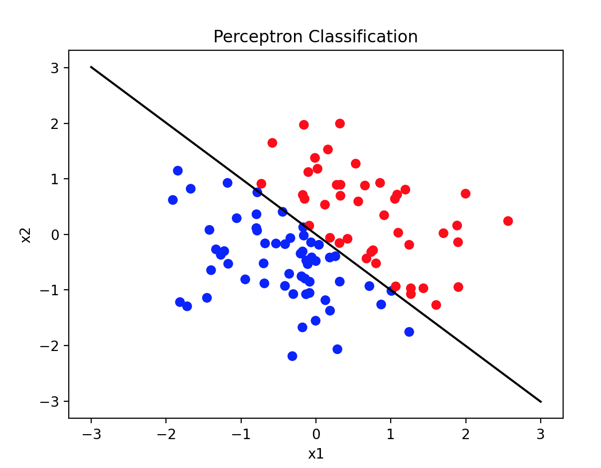
plt.scatter(X[:, 0], X[:, 1], c=y, cmap='bwr')
x1 = np.linspace(-3, 3, 100)
x2 = -(perceptron.w[0] * x1 + perceptron.b) / perceptron.w[1]
plt.plot(x1, x2, 'k-')
plt.xlabel('x1')
plt.ylabel('x2')
plt.title('Perceptron Classification')
plt.show()

代码解释

1. 数据生成：generate_data 函数生成随机的二维数据，并根据 \(x_1 + x_2\) 的符号来标记类别。
2. 感知器模型：Perceptron 类实现了感知器模型的训练、预测和评估方法。
3. 数据划分：将生成的数据划分为训练集、验证集和测试集。
4. 模型训练：使用训练集对感知器模型进行训练。
5. 模型验证和测试：使用验证集和测试集评估模型的准确率。
6. 可视化：绘制数据点和决策边界。