决策树与线性回归算法学习

决策树

决策树（Decision Tree），它是一种以树形数据结构来展示决策规则和分类结果的模型，作为一种归纳学习算法，其重点是将看似无序、杂乱的已知数据，通过某种技术手段将它们转化成可以预测未知数据的树状模型。

每一条从根结点（对最终分类结果贡献最大的属性）到叶子结点（最终分类结果）的路径都代表一条决策的规则。如下图。

原理介绍

决策树回归器通过递归地选择最佳特征和分裂点，将数据划分为不同的区域，以最小化每个区域内目标变量的方差。

这里我们以一个例子来简单介绍决策树的原理。

假设我们有以下简化的数据集，用于预测钻石的价格：

carat	depth	table	price
0.5	60.0	55.0	1500
1.0	62.0	57.0	3500
1.5	63.0	58.0	5500
2.0	64.0	59.0	7500

第一步：选择最佳特征和分裂点

• 假设carat是对price影响最大的特征，选择分裂点1.0。
• 数据被分为两部分：
  • carat <= 1.0：价格在1500和3500之间
  • carat > 1.0：价格在5500和7500之间

第二步：对子集继续分裂

• 对于

  carat <= 1.0
  

  的子集，可能选择

  depth
  

  作为最佳特征，分裂点

  60.5
  

  • depth <= 60.5：价格为1500
  • depth > 60.5：价格为3500

• 对于carat > 1.0的子集，继续选择最佳特征和分裂点，直到每个叶节点内的数据方差达到最小或满足其他停止条件。

最终结果：

• 叶节点1：carat <= 1.0且depth <= 60.5，预测价格为1500
• 叶节点2：carat <= 1.0且depth > 60.5，预测价格为3500
• 叶节点3：carat > 1.0且depth <= 63.5，预测价格为5500
• 叶节点4：carat > 1.0且depth > 63.5，预测价格为7500

可视化示意

         carat <= 1.0
            /          \
   depth <= 60.5      depth > 60.5
      /      \            /       \
  1500      3500        5500      7500

sklearn实现决策树

这里以kaggle 上的一个回归问题为例来实现砖石价格的预测:

https://www.kaggle.com/datasets/shivam2503/diamonds

实现代码如下:

# 1、导入数据集
# -- import some packages
# %matplotlib inline
import pandas as pd
import numpy as np
import matplotlib.pyplot as plt

# 0,克拉，切工质量，颜色，净度，深度百分比，台宽，价格，X，Y，Z尺寸(长度、宽度、深度)
# Unnamed: 0,carat,cut,color,clarity,depth,table,price,x,y,z
# 8116,1.01,Ideal,G,SI2,62.1,57.0,4350,6.48,6.44,4.01
# 52452,0.59,Ideal,E,VVS2,61.8,56.0,2515,5.39,5.42,3.34
# 21546,1.02,Ideal,F,VVS1,62.4,56.0,9645,6.44,6.42,4.01
# 9658,1.01,Premium,H,SI1,61.2,58.0,4642,6.47,6.43,3.95


# -- load the data (csv format)
df = pd.read_csv('diamonds.csv', sep = ',')

# -- remove the data samples with missing values (NaN)
df = df.dropna()

# -- drop the column containing the id of the data
df = df.drop(columns=['Unnamed: 0'], axis=1)

# -- print the column names together with their data type
print(df.dtypes)



# -- print the first 5 rows of the dataframe
print(df.head())



# 在下面的单元格中，我们将（pandas）数据框转换为集合X（包含我们的特征）和集合Y（包含我们的目标，即价格）。 # -- compute X and Y sets
X = df.drop(columns=['price'], axis=1)      # 特征
Y = df['price']                             # 价格

print("Total number of samples:", X.shape[0])

# -- 打印特性名称
features_names = list(X.columns)
print("Features names:", features_names)

X = X.values
Y = Y.values

# -- print shapes
print('X shape: ', X.shape)
print('Y shape: ', Y.shape)






# 2、数据预处理
# 2_1、首先打印每个列的数据类型，返回列名及其在X中的对应索引。
# -- print the data type of each column
# for index_col, name_col in zip(range(X.shape[1]), features_names):
#     print(f"Column {name_col} (index: {index_col}) -- data type: {type(X[0, index_col])}")


# 2_2、现在让我们对分类变量进行编码。
from sklearn.preprocessing import OrdinalEncoder
# -- TO DO
# -------------------------------------------------------------------------------------- TO DO1 start
# 就是把分类特征转化为分类数值的过程，只需要转化cut、color、clarity这几个字符串为数字大小即可

categorical_features = ['cut', 'color', 'clarity']
cut_categories = ['Fair', 'Good', 'Very Good', 'Premium', 'Ideal']
color_categories = ['J', 'I', 'H', 'G', 'F', 'E', 'D']
clarity_categories = ['I1', 'SI2', 'SI1', 'VS2', 'VS1', 'VVS2', 'VVS1', 'IF']
categories = [
    cut_categories,
    color_categories,
    clarity_categories
]
categorical_indices = [features_names.index(col) for col in categorical_features]
encoder = OrdinalEncoder(categories=categories)     # 将按照指定的类别顺序进行编码

X[:, categorical_indices] = encoder.fit_transform(X[:, categorical_indices])

# print("\n编码后的前5行:")
# encoded_df = pd.DataFrame(X, columns=features_names)
# print(encoded_df.head())
# -------------------------------------------------------------------------------------- TO DO1 end


# 2_3、检查编码是否正确完成。
# -- 打印每一列的数据类型
# for index_col, name_col in zip(range(X.shape[1]), features_names):
#     print(f"Column {name_col} (index: {index_col}) -- data type: {type(X[0, index_col])}")
    


# 2_4、数据分成 4/5训练集与 1/5 测试集
# -- TO DO
# -------------------------------------------------------------------------------------- TO DO2 begin
print("Amount of data for training and deciding parameters:",4 / 5*X.shape[0] )
print("Amount of data for test:", 1/5 * X.shape[0])
# -------------------------------------------------------------------------------------- TO DO2 end



# -- TO DO
# -------------------------------------------------------------------------------------- TO DO3 begin
from sklearn.model_selection import train_test_split
# 分割数据集为训练集和测试集，测试集占20%
X_train, X_test, Y_train, Y_test = train_test_split(            # Y_train, Y_test  类似于之前的标签，用来测试准确度的
    X, Y, 
    test_size=0.2,       # 测试集比例为20%
    random_state=42      # 设置随机种子以保证结果可复现
)

# -------------------------------------------------------------------------------------- TO DO3 end



# 2_5、数据标准化
# 注意：只标准化6个连续变量(carat,.depth,table,x,y,z),而不是刚刚编码的3个分类变量。
# 这一步是按标准正态分布进行标准化，不过没有使用归一化
# -- TO DO
# -------------------------------------------------------------------------------------- TO DO4 begin
from sklearn.preprocessing import StandardScaler
import copy

numerical_features = ['carat', 'depth', 'table', 'x', 'y', 'z']
numerical_indices = [features_names.index(col) for col in numerical_features]

scaler = StandardScaler()


X_train_scaled = copy.deepcopy(X_train)
X_test_scaled = copy.deepcopy(X_test)



# 拟合 StandardScaler 
scaler.fit(X_train_scaled[:, numerical_indices])

X_train_scaled[:, numerical_indices] = scaler.transform(X_train_scaled[:, numerical_indices])
X_test_scaled[:, numerical_indices] = scaler.transform(X_test_scaled[:, numerical_indices])


# # 检测、查看标准化后的前5行数据
# print("\n标准化后的训练集前5行:")
# encoded_features = [col for col in features_names if col not in numerical_features]

# scaled_df = pd.DataFrame(X_train_scaled, columns=features_names)
# print(scaled_df.head())

# -------------------------------------------------------------------------------------- TO DO4 end




# 3、构造决策树模型
# 3_1、默认设置
# -- TO DO
# -------------------------------------------------------------------------------------- TO DO5 begin
from sklearn.tree import DecisionTreeRegressor
# -- TO DO
model = DecisionTreeRegressor(random_state=111)


model.fit(X_train_scaled, Y_train)
r2_train = model.score(X_train_scaled, Y_train)
r2_test = model.score(X_test_scaled, Y_test)

one_minus_r2_train = 1 - r2_train
one_minus_r2_test = 1 - r2_test


print("1 - coefficient of determination on training data:", one_minus_r2_train)
print("1 - coefficient of determination on test data:", one_minus_r2_test)


# 获取决策树的深度和节点数量
max_depth = model.tree_.max_depth
node_count = model.tree_.node_count
print("Depth of the tree:", max_depth)
print("Number of nodes:", node_count)

预测结果还是挺不错的:

Amount of data for training and deciding parameters: 6400.0
Amount of data for test: 1600.0
1 - coefficient of determination on training data: 5.2504353975635354e-08
1 - coefficient of determination on test data: 0.054085953341423076
Depth of the tree: 26
Number of nodes: 11905

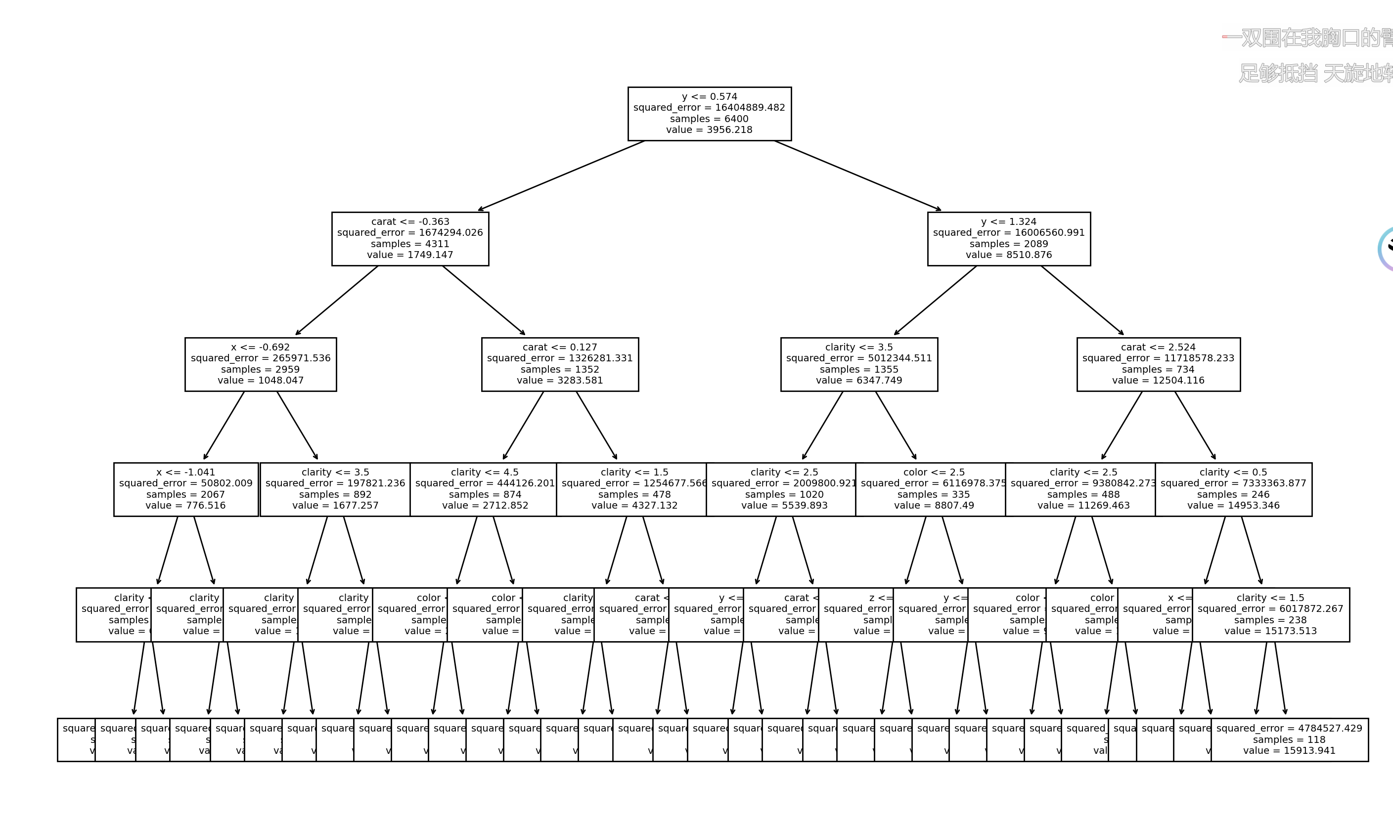
绘出max_depth=5时的决策树图片

from sklearn.tree import DecisionTreeRegressor
# 初始化决策树回归模型，设置 max_depth=5 和 random_state 为学号
model = DecisionTreeRegressor(max_depth=5, random_state=111)

model.fit(X_train_scaled, Y_train)

r2_train = model.score(X_train_scaled, Y_train)
r2_test = model.score(X_test_scaled, Y_test)

one_minus_r2_train = 1 - r2_train
one_minus_r2_test = 1 - r2_test

# -- print the value of 1 - coefficient of determination R^2, for the training and test data
print("1 - coefficient of determination on training data:", one_minus_r2_train)
print("1 - coefficient of determination on test data:", one_minus_r2_test)

# 绘制决策树
from sklearn import tree
import matplotlib.pyplot as plt

plt.figure(figsize=(20,10))  # 设置图形尺寸为20x10英寸
tree.plot_tree(
    decision_tree=model, 
    feature_names=features_names, 
    class_names=['price'],
    fontsize=7              # 设置字体大小
)

plt.savefig('tree.pdf')
plt.show()

K折交叉验证 + max_depth调优

from sklearn.tree import DecisionTreeRegressor
from sklearn.model_selection import KFold
import numpy as np
import matplotlib.pyplot as plt
from sklearn import tree

numero_di_matricola = numero_di_matricola  # e.g., 20231234

# Define the grid for the max_depth hyperparameter (1 to 30 inclusive)
max_depth_grid = list(range(1, 31))


err_train_kfold = []
err_val_kfold = []

kf = KFold(n_splits=5, shuffle=True, random_state=numero_di_matricola)


for depth in max_depth_grid:
    train_errors = []
    val_errors = []
    
    for train_index, val_index in kf.split(X_train_scaled):
        X_train_fold, X_val_fold = X_train_scaled[train_index], X_train_scaled[val_index]
        Y_train_fold, Y_val_fold = Y_train[train_index], Y_train[val_index]
        
        model = DecisionTreeRegressor(max_depth=depth, random_state=numero_di_matricola)
        model.fit(X_train_fold, Y_train_fold)
        
        r2_train = model.score(X_train_fold, Y_train_fold)
        r2_val = model.score(X_val_fold, Y_val_fold)
        
        train_errors.append(1 - r2_train)
        val_errors.append(1 - r2_val)
    
    # 算平均值
    avg_train_error = np.mean(train_errors)
    avg_val_error = np.mean(val_errors)
    
    
    err_train_kfold.append(avg_train_error)
    err_val_kfold.append(avg_val_error)

# Choose the max_depth that minimizes the validation error
min_val_error = min(err_val_kfold)
max_depth_opt = max_depth_grid[err_val_kfold.index(min_val_error)]

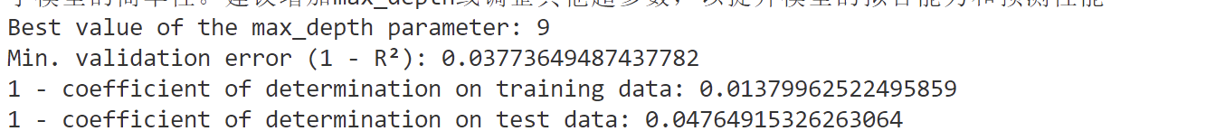
print('Best value of the max_depth parameter:', max_depth_opt)
print('Min. validation error (1 - R²):', min_val_error)


# 3_5_2、画图展示 不同max_depth下的调优效果
# Plot validation and training error (1 - R²) for different values of max_depth
plt.figure(figsize=(10, 6))
plt.plot(max_depth_grid, err_train_kfold, color='r', marker='x', label='training error')
plt.plot(max_depth_grid, err_val_kfold, color='b', marker='x', label='validation error')

# 突出最优值的地方
plt.scatter(max_depth_opt, min_val_error, color='b', marker='o', s=100, label='best max_depth')

plt.legend()
plt.xlabel('max_depth')
plt.ylabel('Error (1 - R²)')
plt.title('DecisionTreeRegressor: Selection of max_depth Parameter')
plt.grid(True)
plt.savefig('train_val_loss.pdf')
# plt.show()

# 3_5_3、使用上面得到的最优 max_depth 学习最终训练模型，并打印 1-R²
final_model = DecisionTreeRegressor(max_depth=max_depth_opt, random_state=numero_di_matricola)
final_model.fit(X_train_scaled, Y_train)

# Calculate R² for training and test sets
r2_train_final = final_model.score(X_train_scaled, Y_train)
r2_test_final = final_model.score(X_test_scaled, Y_test)

# Calculate 1 - R²
one_minus_r2_train_final = 1 - r2_train_final
one_minus_r2_test_final = 1 - r2_test_final

print("1 - coefficient of determination on training data:", one_minus_r2_train_final)
print("1 - coefficient of determination on test data:", one_minus_r2_test_final)

# -------------------------------------------------------------------------------------- TO DO9 end

可以找到最优的max_depth值:

下面打印最优max_depth下的前三重要的宝石特征:

import numpy as np

print(final_model.feature_importances_)  # -- TO DO

top3_idx = np.argsort(final_model.feature_importances_)[-3:][::-1]  # -- TO DO

# 打印这三个特征的名称和索引
print("\nTop 3 most important features:")
for idx in top3_idx:
    print(f"==>\t{features_names[idx]} {idx}")  # -- TO DO

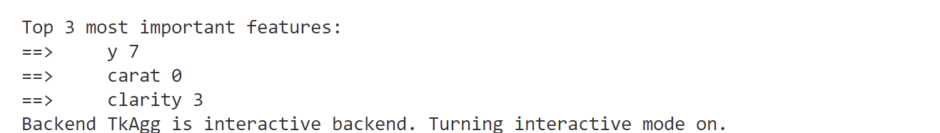
出乎意料的，居然是y、carat、clarity这三个！

线性回归

原理

• 类似于这种的，都是线性回归模型:

  \(h_{\theta}(x)=\theta_{0}+\theta_{1} x_{1}+\theta_{2} x_{2}+\ldots+\theta_{n} x_{n}\)

  \(h_{\theta}(x)=\theta_{0}+\theta_{1} x_{1}+\theta_{2} x_{2}^{2}+\theta_{3} x_{3}^{3}\)

• 线性回归的优化算法也是依靠最小二乘法与梯度下降算法。

  这两个算法，我在神经网络的文章中已经讲过了，不再赘述。

sklearn实现线性回归

还是宝石样本

一阶多项式训练模型

这里使用了默认的模型，即 \(y=\beta_0+\beta_1x_1+\beta_2x_2+\ldots+\beta_px_p+\epsilon\)

# 1、导入数据集
import pandas as pd
import numpy as np
import matplotlib.pyplot as plt

df = pd.read_csv('diamonds.csv', sep = ',')
df = df.dropna()
df = df.drop(columns=['Unnamed: 0'], axis=1)

X = df.drop(columns=['price'], axis=1)      # 特征
Y = df['price']                             # 价格

features_names = list(X.columns)

X = X.values
Y = Y.values

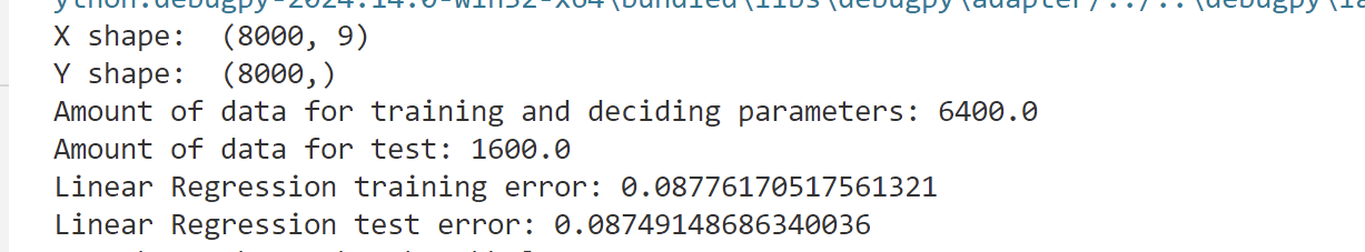
print('X shape: ', X.shape)
print('Y shape: ', Y.shape)

# 2、预处理数据集
# 现在让我们对分类变量进行编码。
from sklearn.preprocessing import OrdinalEncoder
# 就是把分类特征转化为分类数值的过程，只需要转化cut、color、clarity这几个字符串为数字大小即可

categorical_features = ['cut', 'color', 'clarity']
cut_categories = ['Fair', 'Good', 'Very Good', 'Premium', 'Ideal']
color_categories = ['J', 'I', 'H', 'G', 'F', 'E', 'D']
clarity_categories = ['I1', 'SI2', 'SI1', 'VS2', 'VS1', 'VVS2', 'VVS1', 'IF']
categories = [
    cut_categories,
    color_categories,
    clarity_categories
]
categorical_indices = [features_names.index(col) for col in categorical_features]
encoder = OrdinalEncoder(categories=categories)     # 将按照指定的类别顺序进行编码

X[:, categorical_indices] = encoder.fit_transform(X[:, categorical_indices])

# print("\n编码后的前5行:")
# encoded_df = pd.DataFrame(X, columns=features_names)
# print(encoded_df.head())


# 数据分成 4/5训练集与 1/5 测试集
print("Amount of data for training and deciding parameters:",4 / 5*X.shape[0] )
print("Amount of data for test:", 1/5 * X.shape[0])


from sklearn.model_selection import train_test_split
# 分割数据集为训练集和测试集，测试集占20%
X_train, X_test, Y_train, Y_test = train_test_split(            # Y_train, Y_test  类似于之前的标签，用来测试准确度的
    X, Y, 
    test_size=0.2,       # 测试集比例为20%
    random_state=42      # 设置随机种子以保证结果可复现
)


from sklearn.preprocessing import StandardScaler
import copy

numerical_features = ['carat', 'depth', 'table', 'x', 'y', 'z']
numerical_indices = [features_names.index(col) for col in numerical_features]

scaler = StandardScaler()


X_train_scaled = copy.deepcopy(X_train)
X_test_scaled = copy.deepcopy(X_test)

# 拟合 StandardScaler 
scaler.fit(X_train_scaled[:, numerical_indices])

X_train_scaled[:, numerical_indices] = scaler.transform(X_train_scaled[:, numerical_indices])
X_test_scaled[:, numerical_indices] = scaler.transform(X_test_scaled[:, numerical_indices])



# 3、下面才是 线性回归的关键函数
from sklearn.linear_model import LinearRegression

# 初始化并训练线性回归模型
lr_model = LinearRegression()
lr_model.fit(X_train_scaled, Y_train)

# 计算训练集和测试集上的R²分数
r2_train_lr = lr_model.score(X_train_scaled, Y_train)
r2_test_lr = lr_model.score(X_test_scaled, Y_test)



print("Linear Regression training error:", 1 - r2_train_lr)
print("Linear Regression test error:", 1 - r2_test_lr)

二阶多项式训练模型

下面使用 二阶多项式 来训练模型

# 1、导入必要的库
import pandas as pd
import matplotlib.pyplot as plt
from sklearn.preprocessing import OrdinalEncoder, StandardScaler, PolynomialFeatures
from sklearn.model_selection import train_test_split
from sklearn.linear_model import LinearRegression


import pandas as pd
import numpy as np
import matplotlib.pyplot as plt

df = pd.read_csv('diamonds.csv', sep = ',')
df = df.dropna()
df = df.drop(columns=['Unnamed: 0'], axis=1)

X = df.drop(columns=['price'], axis=1)      # 特征
Y = df['price']                             # 价格

features_names = list(X.columns)

X = X.values
Y = Y.values

print('X shape: ', X.shape)
print('Y shape: ', Y.shape)

# 2、预处理数据集
# 现在让我们对分类变量进行编码。
from sklearn.preprocessing import OrdinalEncoder
# 就是把分类特征转化为分类数值的过程，只需要转化cut、color、clarity这几个字符串为数字大小即可

categorical_features = ['cut', 'color', 'clarity']
cut_categories = ['Fair', 'Good', 'Very Good', 'Premium', 'Ideal']
color_categories = ['J', 'I', 'H', 'G', 'F', 'E', 'D']
clarity_categories = ['I1', 'SI2', 'SI1', 'VS2', 'VS1', 'VVS2', 'VVS1', 'IF']
categories = [
    cut_categories,
    color_categories,
    clarity_categories
]
categorical_indices = [features_names.index(col) for col in categorical_features]
encoder = OrdinalEncoder(categories=categories)     # 将按照指定的类别顺序进行编码

X[:, categorical_indices] = encoder.fit_transform(X[:, categorical_indices])




# 数据分成 4/5训练集与 1/5 测试集
print("Amount of data for training and deciding parameters:",4 / 5*X.shape[0] )
print("Amount of data for test:", 1/5 * X.shape[0])


from sklearn.model_selection import train_test_split
# 分割数据集为训练集和测试集，测试集占20%
X_train, X_test, Y_train, Y_test = train_test_split(            # Y_train, Y_test  类似于之前的标签，用来测试准确度的
    X, Y, 
    test_size=0.2,       # 测试集比例为20%
    random_state=42      # 设置随机种子以保证结果可复现
)



# 3、使用 二阶多项式 来进行训练模型
# 创建多项式特征生成器，degree=2表示二阶多项式
poly = PolynomialFeatures(degree=2, include_bias=False, interaction_only=False)

X_train_poly = poly.fit_transform(X_train)
X_test_poly = poly.transform(X_test)

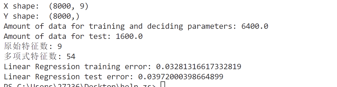
poly_features = poly.get_feature_names_out(features_names)
print("原始特征数:", X_train.shape[1])
print("多项式特征数:", X_train_poly.shape[1])

# 训练线性回归模型
lr_model_poly = LinearRegression()
lr_model_poly.fit(X_train_poly, Y_train)

# 计算训练集和测试集上的R²分数
r2_train_lr_poly = lr_model_poly.score(X_train_poly, Y_train)
r2_test_lr_poly = lr_model_poly.score(X_test_poly, Y_test)

print("Linear Regression training error:", 1 - r2_train_lr_poly)
print("Linear Regression test error:", 1 - r2_test_lr_poly)

可以发现结果好很多

优缺点

优点:

• 思想简单，实现容易。建模迅速，对于小数据量、简单的关系很有效。
• 结果具有很好的可解释性，有利于决策分析。
• 能解决回归问题。

缺点:

• 对于非线性数据或者数据特征间具有相关性多项式回归难以建模.
• 难以很好地表达高度复杂的数据。