
一、选题背景:
景观识别是一种人工智能技术,旨在通过自然场景的图像或视频来识别和分类不同的景观类型。这种技术可以用于多种应用场景,如旅游、地理信息系统、环境监测等。
在地理信息系统领域,景观识别技术可以帮助收集和维护地理信息数据,例如道路、建筑物、植被等。在环境监测领域,景观识别技术可以帮助监测和分析自然环境的变化,例如森林覆盖率、植被生长情况等。
景观识别技术的研究对象主要是自然场景,包括冰川、山脉、沙漠、海滩、森林等。
二、机器学习设计方案:
网站中下载相关的数据集,对数据集进行整理,在python的环境中,给数据集中的文件打上标签,对数据进行预处理,利用keras,构建网络,训练模型,导入图片测试模型
本题采用的数据集来源于kaggle:https://www.kaggle.com/datasets/
三、机器学习的实现步骤:
1.目的:通过机器学习分别识别出海滩,冰川,森林,沙漠,山脉五个景观图片。
2.下载数据集:
3.导入需要的库
import numpy as np
import pandas as pd
import os
import tensorflow as tf
import matplotlib.pyplot as plt
from pathlib import Path
from sklearn.model_selection import train_test_split
from keras.models import Sequential
from keras.layers import Activation
from keras.layers import Dense, Dropout, Flatten, Conv2D, MaxPooling2D
from keras.applications.resnet import preprocess_input
from keras_preprocessing.image import ImageDataGenerator
from keras.models import load_model
from keras import optimizers
from keras.utils.np_utils import *
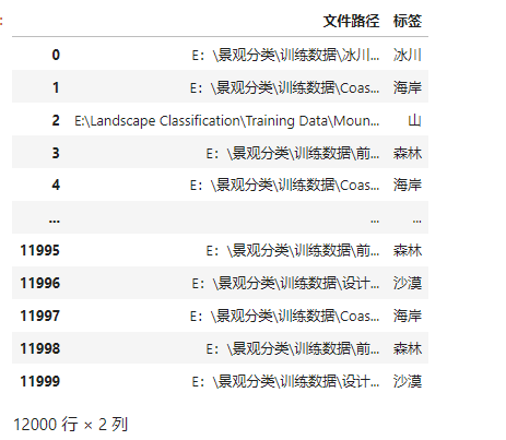
4.遍历数据集中的文件,将路径数据和标签数据生成DataFrame
dir = Path('E:/Landscape Classification')
# 用glob遍历在dir路径中所有jpg格式的文件,并将所有的文件名添加到filepaths列表中
filepaths = list(dir.glob(r'**/*.jpeg'))
将文件中的分好的小文件名(种类名)分离并添加到labels的列表中
labels = list(map(lambda l: os.path.split(os.path.split(l)[0])[1], filepaths))
将filepaths通过pandas转换为Series数据类型
filepaths = pd.Series(filepaths, name='FilePaths').astype(str)
将labels通过pandas转换为Series数据类型
labels = pd.Series(labels, name='Labels').astype(str)
将filepaths和Series两个Series的数据类型合成DataFrame数据类型
df = pd.merge(filepaths, labels, right_index=True, left_index=True)
df = df[df['Labels'].apply(lambda l: l[-2:] != 'GT')]
df = df.sample(frac=1).reset_index(drop=True)#查看形成的DataFrame的数据df
df
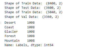
5.将原始数据按照一定的比例分成训练集、验证集和测试集。
X_train, X_test = train_test_split(df, test_size=0.3, stratify=df['Labels'])

print('Shape of Train Data: ', X_train.shape)
print('Shape of Test Data: ', X_test.shape)


X_train, X_val = train_test_split(X_train, test_size=0.4, stratify=X_train['Labels'])

print('Shape of Train Data: ', X_train.shape)
print('Shape of Val Data: ', X_val.shape)

# 查看各个标签的图片张数
X_train['Labels'].value_counts(ascending=True)
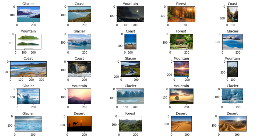
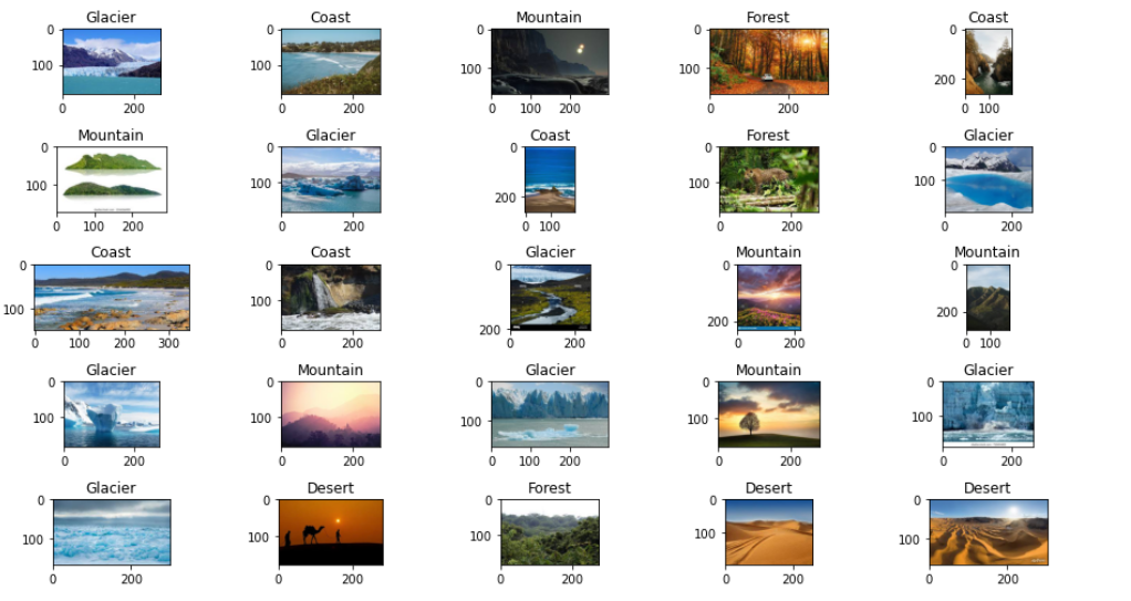
6.绘出图像和图像标签
#创建一个包含 5 行 5 列的图像的绘图窗口
fit, ax = plt.subplots(nrows=5, ncols=5, figsize=(13, 7))
for i, a in enumerate(ax.flat):#遍历子图
    a.imshow(plt.imread(df.FilePaths[i]))
    a.set_title(df.Labels[i])

plt.tight_layout()
plt.show()
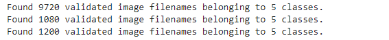
7.创建一个图像生成器,用于生成训练、验证和测试数据。
# 批量的大小
BATCH_SIZE = 32
# 输入图片的大小
IMG_SIZE = (150, 150)

# 使用preprocessing_function参数指定了一个预处理函数,该函数用于将输入图像进行预处理,使其符合模型的输入格式。
img_data_gen = ImageDataGenerator(preprocessing_function=preprocess_input)
X_train = img_data_gen.flow_from_dataframe(dataframe=X_train,
                                          x_col='FilePaths',#参数指定了数据中包含图像路径的列名
                                          y_col='Labels',#参数指定了数据帧中包含图像标签的列名
                                          target_size=IMG_SIZE,#参数指定了图像的大小
                                          color_mode='rgb',#参数指定了图像的rgb颜色模式
                                          class_mode='categorical',#参数指定了图像的分类模式,多类别
                                          batch_size=BATCH_SIZE,#参数指定了生成器生成的每个批次的大小
                                          seed=42)#参数指定了随机数生成器的种子,用于生成随机打乱的数据。

X_val = img_data_gen.flow_from_dataframe(dataframe=X_val,
                                          x_col='FilePaths',
                                          y_col='Labels',
                                          target_size=IMG_SIZE,
                                          color_mode='rgb',
                                          class_mode='categorical',
                                          batch_size=BATCH_SIZE,
                                          seed=42)
X_test = img_data_gen.flow_from_dataframe(dataframe=X_test,
                                          x_col='FilePaths',
                                          y_col='Labels',
                                          target_size=IMG_SIZE,
                                          color_mode='rgb',
                                          class_mode='categorical',
                                          batch_size=BATCH_SIZE,
                                          seed=42)
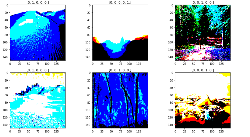
8.绘出经过处理的图像和 图像标签索引,用于后面预测时对应创建字典的值
fit, ax = plt.subplots(nrows=2, ncols=3, figsize=(13,7))

for i, a in enumerate(ax.flat):
    img, label = X_train.next()
    a.imshow(img[0],)
    a.set_title(label[0])
plt.tight_layout()
plt.show()
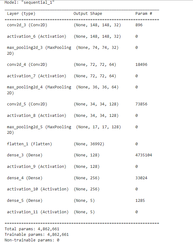
9.创建卷积神经网络模型
#创建输入层,卷积层,池化层,全连接层,输出层
model = Sequential()

# 1层

#Output shape计算公式:(150-3+1=148
#param参数数量:32*3*3*3+32=896
model.add(Conv2D(
    filters=32, #卷积核个数32个
    kernel_size= (3,3) ,
    input_shape=(150,150,3) ,
))
model.add(Activation('relu'))
model.add(MaxPooling2D(
    pool_size=(2,2), # 输出图片尺寸:148/2=74*74
    strides=2,
))
#CNN 2层
model.add(Conv2D(
    filters=64,  #Output (50,50,64)
    kernel_size=(3,3),
))
model.add(Activation('relu'))
model.add(MaxPooling2D(  #Output(25,25,64)
    pool_size=(2,2),
    strides=2,
))

#CNN 3层
model.add(Conv2D(
    filters=128,  #Output (50,50,64)
    kernel_size=(3,3),
))
model.add(Activation('relu'))
model.add(MaxPooling2D(  #Output(25,25,64)
    pool_size=(2,2),
    strides=2,
))
#全连层1
model.add(Flatten())
model.add(Dense(128))
model.add(Activation('relu'))

#全连层2
model.add(Dense(256))
model.add(Activation('relu'))

model.add(Dense(5))#添加5个节点的连接层
model.add(Activation('softmax'))#添加激活层,softmax将输入的一个向量转换为概率分布


#编译模型
model.compile(optimizer=optimizers.RMSprop(lr=1e-4),
               loss="categorical_crossentropy",
               metrics=["accuracy"])
model.summary()
#训练模型
h1 = model.fit(X_train, validation_data=X_val,
               epochs=30, )
#保存模型
model.save('lwl41.h5')
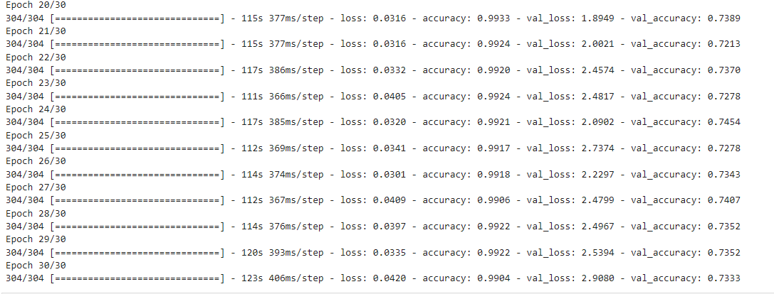
10.绘制训练过程中模型的准确率和损失的变化曲线
accuracy = h1.history['accuracy']
loss = h1.history['loss']
val_loss = h1.history['val_loss']
val_accuracy = h1.history['val_accuracy']
plt.figure(figsize=(17, 7))
plt.subplot(2, 2, 1)
plt.plot(range(30), accuracy,'bo', label='Training Accuracy')
plt.plot(range(30), val_accuracy, label='Validation Accuracy')
plt.legend(loc='lower right')
plt.title('Accuracy : Training vs. Validation ')
plt.subplot(2, 2, 2)
plt.plot(range(30), loss,'bo' ,label='Training Loss')
plt.plot(range(30), val_loss, label='Validation Loss')
plt.title('Loss : Training vs. Validation ')
plt.legend(loc='upper right')
plt.show()
从图分析,这种情况可能是由于模型过度拟合训练数据而导致的,导致它在训练数据上表现良好,但是在验证数数上表现不佳。
11.通过ImageDataGenerator数据增强器,训练数据中进行随机变换的方式,帮助模型学习更多的特征,来降低过拟合
#修改预处理图像中ImageDataGenerator的参数,实现数据增强
img_data_gen = ImageDataGenerator(rescale=1./255,
                                  rotation_range=50, #将图像随机旋转50度
                                  width_shift_range=0.3, #在水平方向上平移比例为0.
                                  height_shift_range=0.3, #在垂直方向上平移比例为0.3
                                  shear_range=0.3, #随机错切变换的角度为0.3
                                  zoom_range=0.3, #图片随机缩放的范围为0.3
                                  horizontal_flip=True, #随机将一半图像水平翻转
                                  fill_mode='nearest')
在重新进行训练和绘制损失曲线和精度曲线图
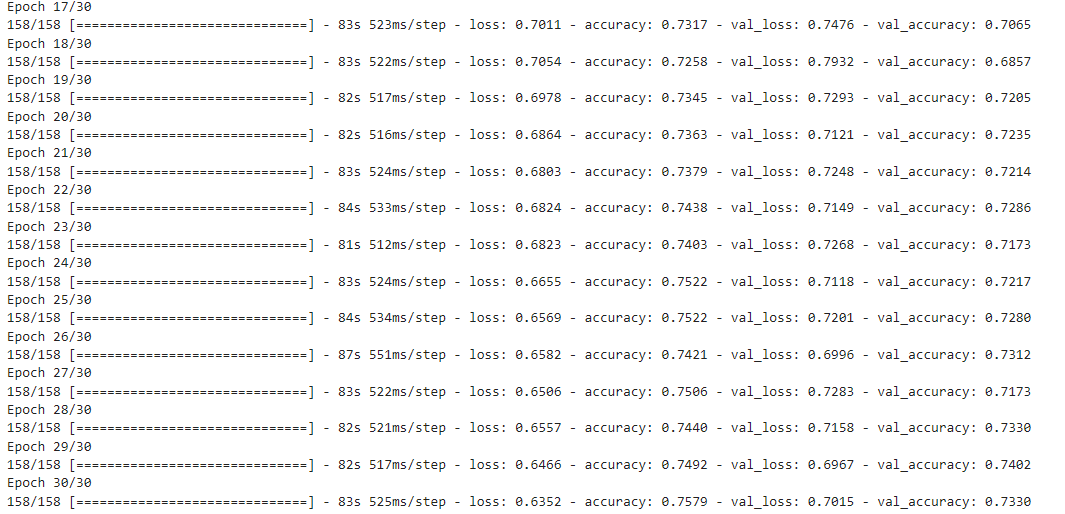

发现过拟合的情况已经有效的解决了。
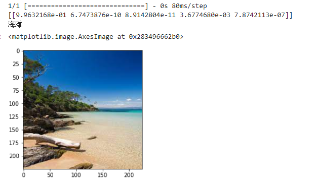
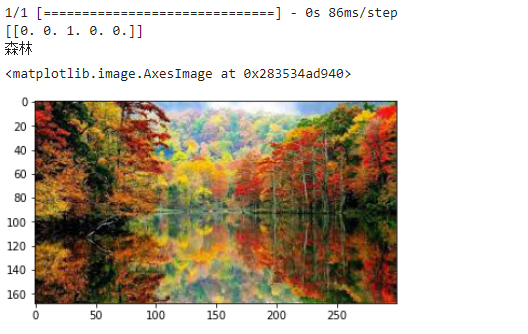
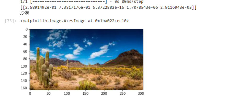
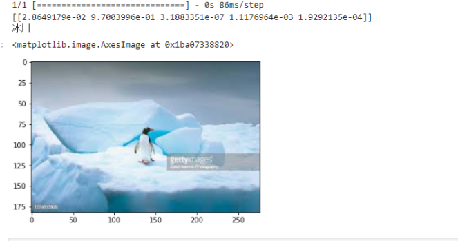
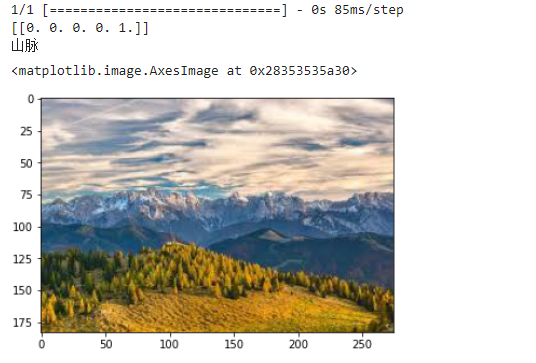
12.导入图片进行预测
from PIL import Image
from keras.utils import image_utils
def con(file,outdir,w=150,h=150):
    img1=Image.open(file)
    img2=img1.resize((w,h),Image.BILINEAR)
    img2.save(os.path.join(outdir,os.path.basename(file)))
file='E:/Landscape Classification/Testing Data/Mountain/Mountain-Test (7).jpeg'
con(file,'E:/')
model=load_model('lwl41.h5')
img_path='E:/Landscape Classification/Testing Data/Mountain/Mountain-Test (7).jpeg'
img = image_utils.load_img(img_path,target_size=(150,150))
img = image_utils.img_to_array(img)
img = np.expand_dims(img, axis=0)
out = model.predict(img)
print(out)
dict={'0':'海滩','1':'冰川','2':'森林','3':'沙漠','4':'山脉'}
for i in range(5):
    if out[0][i]>0.5:
        print(dict[str(i)])
img=plt.imread('E:/Landscape Classification/Testing Data/Mountain/Mountain-Test (7).jpeg')
plt.imshow(img)
完整代码附上:
点击查看代码
#导入需要用到的库
import numpy as np
import pandas as pd
import os
import tensorflow as tf
import matplotlib.pyplot as plt
from pathlib import Path
from sklearn.model_selection import train_test_split
from keras.models import Sequential
from keras.layers import Activation
from keras.layers import Dense, Dropout, Flatten, Conv2D, MaxPooling2D
from keras.applications.resnet import preprocess_input
from keras_preprocessing.image import ImageDataGenerator
from keras.models import load_model
from keras import optimizers
from keras.utils.np_utils import *

dir = Path('E:/Landscape Classification')

# 用glob遍历在dir路径中所有jpg格式的文件,并将所有的文件名添加到filepaths列表中
filepaths = list(dir.glob(r'**/*.jpeg'))

# 将文件中的分好的小文件名(种类名)分离并添加到labels的列表中
labels = list(map(lambda l: os.path.split(os.path.split(l)[0])[1], filepaths))

# 将filepaths通过pandas转换为Series数据类型
filepaths = pd.Series(filepaths, name='FilePaths').astype(str)

# 将labels通过pandas转换为Series数据类型
labels = pd.Series(labels, name='Labels').astype(str)

# 将filepaths和Series两个Series的数据类型合成DataFrame数据类型
df = pd.merge(filepaths, labels, right_index=True, left_index=True)
df = df[df['Labels'].apply(lambda l: l[-2:] != 'GT')]
df = df.sample(frac=1).reset_index(drop=True)#查看形成的DataFrame的数据df
df


X_train, X_test = train_test_split(df, test_size=0.3, stratify=df['Labels'])

print('Shape of Train Data: ', X_train.shape)
print('Shape of Test Data: ', X_test.shape)


X_train, X_val = train_test_split(X_train, test_size=0.4,stratify=X_train['Labels'])

print('Shape of Train Data: ', X_train.shape)
print('Shape of Val Data: ', X_val.shape)

# 查看各个标签的图片张数
X_train['Labels'].value_counts(ascending=True)

fit, ax = plt.subplots(nrows=5, ncols=5, figsize=(13, 7))

for i, a in enumerate(ax.flat):
    a.imshow(plt.imread(df.FilePaths[i]))
    a.set_title(df.Labels[i])

plt.tight_layout()
plt.show()

# 批量的大小
BATCH_SIZE = 32
# 输入图片的大小
IMG_SIZE = (150, 150)

# 使用preprocessing_function参数指定了一个预处理函数,该函数用于将输入图像进行预处理,使其符合模型的输入格式。
img_data_gen = ImageDataGenerator(rescale=1./255,
                                  rotation_range=50, #将图像随机旋转50度
                                  width_shift_range=0.3, #在水平方向上平移比例为0.3
                                  height_shift_range=0.3, #在垂直方向上平移比例为0.3
                                  shear_range=0.3, #随机错切变换的角度为0.3
                                  zoom_range=0.3, #图片随机缩放的范围为0.3
                                  horizontal_flip=True, #随机将一半图像水平翻转
                                  fill_mode='nearest')
X_train = img_data_gen.flow_from_dataframe(dataframe=X_train,
                                          x_col='FilePaths',#参数指定了数据中包含图像路径的列名
                                          y_col='Labels',#参数指定了数据帧中包含图像标签的列名
                                          target_size=IMG_SIZE,#参数指定了图像的大小
                                          color_mode='rgb',#参数指定了图像的rgb颜色模式
                                          class_mode='categorical',#参数指定了图像的分类模式,多类别
                                          batch_size=BATCH_SIZE,#参数指定了生成器生成的每个批次的大小
                                          seed=42)#参数指定了随机数生成器的种子,用于生成随机打乱的数据。

X_val = img_data_gen.flow_from_dataframe(dataframe=X_val,
                                          x_col='FilePaths',
                                          y_col='Labels',
                                          target_size=IMG_SIZE,
                                          color_mode='rgb',
                                          class_mode='categorical',
                                          batch_size=BATCH_SIZE,
                                          seed=42)
X_test = img_data_gen.flow_from_dataframe(dataframe=X_test,
                                          x_col='FilePaths',
                                          y_col='Labels',
                                          target_size=IMG_SIZE,
                                          color_mode='rgb',
                                          class_mode='categorical',
                                          batch_size=BATCH_SIZE,
                                          seed=42)

#查看经过处理的图片以及它的binary标签
fit, ax = plt.subplots(nrows=2, ncols=3, figsize=(13,7))

for i, a in enumerate(ax.flat):
    img, label = X_train.next()
    a.imshow(img[0],)
    a.set_title(label[0])

plt.tight_layout()
plt.show()

#-- 创建卷积神经网络

#创建输入层,卷积层,池化层,全连接层,输出层
model = Sequential()

# 1层

#Output shape计算公式:(150-3+1=148
#param参数数量:32*3*3*3+32=896
model.add(Conv2D(
    filters=32, #卷积核个数32个
    kernel_size= (3,3) ,
    input_shape=(150,150,3) ,
))
model.add(Activation('relu'))
model.add(MaxPooling2D(
    pool_size=(2,2), # 输出图片尺寸:148/2=74*74
    strides=2,
))
#CNN 2层
model.add(Conv2D(
    filters=64,  #Output (50,50,64)
    kernel_size=(3,3),
))
model.add(Activation('relu'))
model.add(MaxPooling2D(  #Output(25,25,64)
    pool_size=(2,2),
    strides=2,
))

#CNN 3层
model.add(Conv2D(
    filters=128,  #Output (50,50,64)
    kernel_size=(3,3),
))
model.add(Activation('relu'))
model.add(MaxPooling2D(  #Output(25,25,64)
    pool_size=(2,2),
    strides=2,
))
#全连层1
model.add(Flatten())
model.add(Dense(128))
model.add(Activation('relu'))

#全连层2
model.add(Dense(256))
model.add(Activation('relu'))

model.add(Dense(5))#添加5个节点的连接层
model.add(Activation('softmax'))#添加激活层,softmax将输入的一个向量转换为概率分布


#编译模型
model.compile(optimizer=optimizers.RMSprop(lr=1e-4),
               loss="categorical_crossentropy",
               metrics=["accuracy"])
model.summary()

#训练模型
h1 = model.fit(X_train, validation_data=X_val,
               epochs=30, )
#保存模型
model.save('lwl41.h5')

#绘制损失和精度曲线图
accuracy = h1.history['accuracy']
loss = h1.history['loss']
val_loss = h1.history['val_loss']
val_accuracy = h1.history['val_accuracy']
plt.figure(figsize=(17, 7))
plt.subplot(2, 2, 1)
plt.plot(range(30), accuracy,'bo', label='Training Accuracy')
plt.plot(range(30), val_accuracy, label='Validation Accuracy')
plt.legend(loc='lower right')
plt.title('Accuracy : Training vs. Validation ')
plt.subplot(2, 2, 2)
plt.plot(range(30), loss,'bo' ,label='Training Loss')
plt.plot(range(30), val_loss, label='Validation Loss')
plt.title('Loss : Training vs. Validation ')
plt.legend(loc='upper right')
plt.show()

#预测
from PIL import Image
from keras.utils import image_utils
def con(file,outdir,w=150,h=150):
    img1=Image.open(file)
    img2=img1.resize((w,h),Image.BILINEAR)
    img2.save(os.path.join(outdir,os.path.basename(file)))
file='E:/Landscape Classification/Testing Data/Mountain/Mountain-Test (7).jpeg'
con(file,'E:/')
model=load_model('lwl41.h5')
img_path='E:/Landscape Classification/Testing Data/Mountain/Mountain-Test (7).jpeg'
img = image_utils.load_img(img_path,target_size=(150,150))
img = image_utils.img_to_array(img)
img = np.expand_dims(img, axis=0)
out = model.predict(img)
print(out)
dict={'0':'海滩','1':'冰川','2':'森林','3':'沙漠','4':'山脉'}
for i in range(5):
    if out[0][i]>0.5:
        print(dict[str(i)])
img=plt.imread('E:/Landscape Classification/Testing Data/Mountain/Mountain-Test (7).jpeg')
plt.imshow(img)
总结:
本次机器学习耗时较长时间,中途遇到很多问题,数据集的处理,模型的建立,训练模型过程中出现过拟合,数据增强的应用等等,通过本次课程设计,加深了我对机器学习多分类以及其标签学习的理解,了解了景观识别项目的整体流程,包括数据预处理、训练模型、测试模型等。掌握了数据增强的概念及其在训练模型中的应用方法。
改进建议是:
尽量使用更多的数据,以提高模型的准确性。
尝试使用更多的模型算法,以提高模型的性能。
尝试使用更多的图像预处理技术,来提升模型的性能。
 posted on

 浙公网安备 33010602011771号