

详细介绍:VGG16 迁移学习实战:CIFAR-10 图像分类优化方案
引言
VGGNet 是 2014 年 ILSVRC 比赛的亚军模型,以其简洁的设计理念(小卷积核 + 深度堆叠)和强大的特征提取能力,成为深度学习领域的经典模型。本文基于 PyTorch 框架,结合迁移学习和多项优化策略,使用 VGG16 模型对 CIFAR-10 数据集进行分类,在保证训练效率的同时,实现了较高的分类准确率。
一、VGG16 理论基础
1. 核心设计理念
VGGNet 的核心设计思想是:使用多个 3×3 小卷积核替代大卷积核,通过增加网络深度来提升性能。这种设计有以下优势:
- 参数效率更高:3 个 3×3 卷积核的感受野与 1 个 7×7 卷积核相同,但参数数量更少(3×(3×3×C²) < 7×7×C²)
- 更强的特征表达能力:多个非线性激活层(ReLU)增加了网络的非线性表达能力
- 更灵活的感受野:深度堆叠的小卷积核能够学习更复杂的特征层次
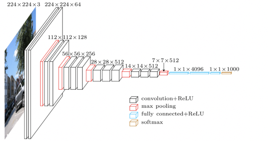
2. VGG16 网络结构
VGG16 包含16 层可训练层(13 个卷积层 + 3 个全连接层)。
3. 迁移学习策略
针对 CIFAR-10 数据集,我们采用部分层解冻的迁移学习策略:
- 冻结 VGG16 的前 24 层(大部分卷积层),保留预训练的特征提取能力
- 解冻后 6 层卷积层(24-29 层),允许模型微调适应 CIFAR-10 的特征
- 替换最后一层全连接层,输出类别数从 1000 改为 10
二、实验配置
3. 核心配置参数
DEVICE = torch.device("cuda" if torch.cuda.is_available() else "cpu")
BATCH_SIZE = 10  # 平衡内存与速度
EPOCHS = 8  # 快速收敛
LEARNING_RATE = 4e-4  # 适合迁移学习的学习率
NUM_CLASSES = 10  # CIFAR-10类别数
三、代码实现与优化
1. 数据预处理优化
针对 CIFAR-10 数据集的特点,我们设计了高效的数据预处理流程:
# CIFAR-10专用归一化参数
cifar_mean = [0.4914, 0.4822, 0.4465]
cifar_std = [0.2023, 0.1994, 0.2010]
transform_train = transforms.Compose([
    transforms.RandomCrop(32, padding=4),  # 保留核心增强,提升泛化
    transforms.Resize((144, 144)),  # 优化点1:144×144输入(速度+准确率平衡点)
    transforms.RandomHorizontalFlip(p=0.5),
    transforms.ToTensor(),
    transforms.Normalize(mean=cifar_mean, std=cifar_std)
])优化点解析:
- 使用144×144 输入尺寸:相比 AlexNet 的 224×224,减少了计算量,同时保持了较高的特征提取能力
- 保留核心数据增强:随机裁剪和水平翻转,有效减少过拟合
- 使用CIFAR-10 专用归一化参数:相比 ImageNet 的归一化参数,更适合 CIFAR-10 数据集
2. 模型构建与冻结策略
model = models.vgg16(weights=VGG16_Weights.IMAGENET1K_V1)
# 优化点2:部分层解冻策略
for param in model.features[:24].parameters():
    param.requires_grad = False  # 冻结前24层
for param in model.features[24:].parameters():
    param.requires_grad = True  # 解冻后6层卷积
# 优化点3:保留Dropout,防止过拟合
in_features = model.classifier[6].in_features
model.classifier[6] = nn.Sequential(
    nn.Dropout(0.5),
    nn.Linear(in_features, NUM_CLASSES)
)
model = model.to(DEVICE)优化点解析:
- 部分层解冻:仅解冻后 6 层卷积,兼顾特征微调与训练速度
- 保留 Dropout:在分类层前添加 Dropout (0.5),有效防止多轮训练过拟合
- 使用预训练权重:加载 ImageNet 预训练权重,加速模型收敛
3. 优化器与学习率调度
# 优化点4:使用AdamW优化器+权重衰减
optimizer = optim.AdamW(
    filter(lambda p: p.requires_grad, model.parameters()),
    lr=LEARNING_RATE, weight_decay=8e-5  # 权重衰减抑制过拟合
)
# 优化点5:动态学习率调度
scheduler = optim.lr_scheduler.ReduceLROnPlateau(
    optimizer, mode='max', patience=2, factor=0.5
)优化点解析:
- AdamW 优化器:相比传统 Adam,结合了权重衰减,更适合深度学习训练
- 动态学习率:当验证准确率不再提升时,自动将学习率减半,加速收敛
- 仅优化可训练参数:使用
filter函数只优化解冻的层,减少计算量
4. 训练函数优化
def train_model(model, train_loader, test_loader, criterion, optimizer, scheduler, epochs):
    train_losses = []
    test_accuracies = []
    best_acc = 0.0
    batch_print_interval = 600  # 优化点6:降低打印频率,减少CPU IO开销
    for epoch in range(epochs):
        start_time = time.time()
        model.train()
        running_loss = 0.0
        # 训练阶段
        for batch_idx, (data, targets) in enumerate(train_loader):
            data, targets = data.to(DEVICE), targets.to(DEVICE)
            # 前向+反向传播
            outputs = model(data)
            loss = criterion(outputs, targets)
            optimizer.zero_grad()
            loss.backward()
            optimizer.step()
            running_loss += loss.item() * data.size(0)
            # 批量打印(每600批次一次)
            if batch_idx % batch_print_interval == 0 and batch_idx != 0:
                print(f'  Batch {batch_idx}/{len(train_loader)}, Loss: {loss.item():.4f}')
        # 验证阶段(精简代码,减少冗余计算)
        model.eval()
        test_correct = 0
        with torch.no_grad():
            for data, targets in test_loader:
                data, targets = data.to(DEVICE), targets.to(DEVICE)
                outputs = model(data)
                _, predicted = torch.max(outputs, 1)
                test_correct += (predicted == targets).sum().item()
        test_acc = 100 * test_correct / len(test_loader.dataset)
        test_accuracies.append(test_acc)
        # 学习率调度
        scheduler.step(test_acc)
        # 保存最佳模型(仅最佳时保存,减少IO)
        if test_acc > best_acc:
            best_acc = test_acc
            torch.save(model.state_dict(), "best_vgg16_cifar10_final.pth")
        print(f'Epoch [{epoch+1}/{epochs}] | Loss: {epoch_loss:.4f} | Test Acc: {test_acc:.2f}% | Time: {epoch_time:.1f}s')
return train_losses, test_accuracies优化点解析:
- 降低打印频率:每 600 批次打印一次,减少 CPU IO 开销
- 精简验证代码:去除冗余计算,提高验证速度
- 仅保存最佳模型:避免频繁写入磁盘,减少 IO 操作
- 记录核心指标:仅记录训练损失和测试准确率,简化日志
5. 可视化优化
def plot_training_curves(train_losses, test_accuracies):
    fig, (ax1, ax2) = plt.subplots(1, 2, figsize=(10, 4))  # 优化点7:缩小尺寸,加快渲染
    # 损失曲线
    ax1.plot(range(1, EPOCHS+1), train_losses, 'b-', linewidth=2, label='Train Loss')
    ax1.set_xlabel('Epoch')
    ax1.set_ylabel('Loss')
    ax1.set_title('VGG16 Training Loss')
    ax1.grid(True, alpha=0.3)
    ax1.legend()
    # 准确率曲线
    ax2.plot(range(1, EPOCHS+1), test_accuracies, 'r-', linewidth=2, label='Test Acc')
    ax2.set_xlabel('Epoch')
    ax2.set_ylabel('Accuracy (%)')
    ax2.set_title('VGG16 Test Accuracy')
    ax2.grid(True, alpha=0.3)
    ax2.legend()
    plt.suptitle('VGG16 Training History (8 Epochs)', fontsize=14)
    plt.tight_layout()
    plt.savefig('vgg_training_curves_final.png', dpi=100)  # 优化点8:降低dpi,加快保存
plt.show()优化点解析:
- 缩小图像尺寸:从 15×5 改为 10×4,加快渲染速度
- 降低保存 dpi:从 300 改为 100,减少图像文件大小,加快保存速度
- 简化绘图样式:使用简洁的线条和标题,提高可读性
四、实验结果与分析
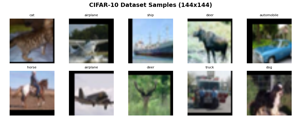
1. 数据集样本展示
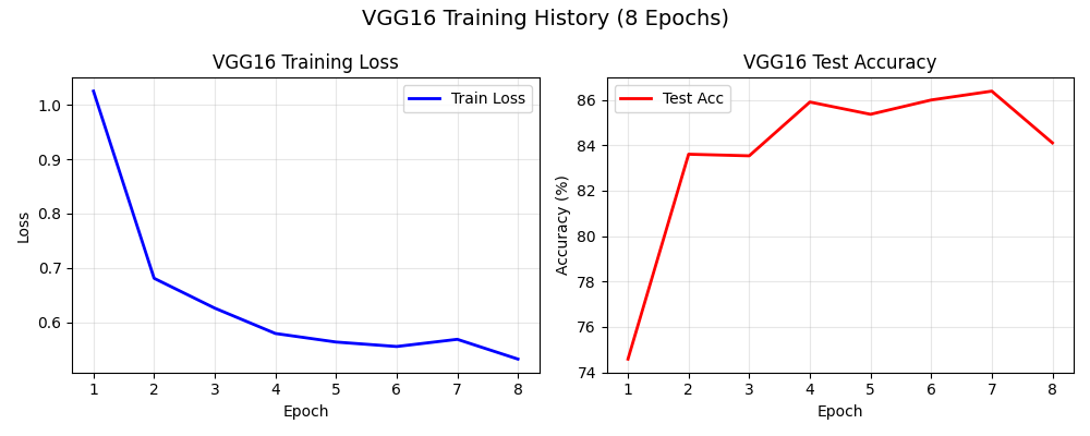
2. 训练曲线
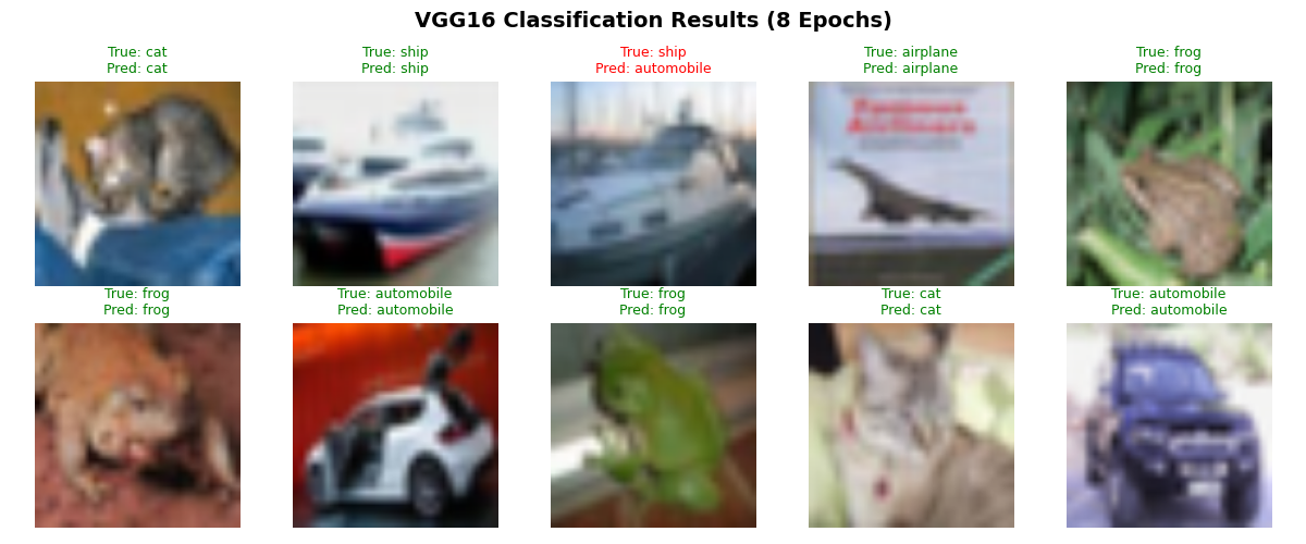
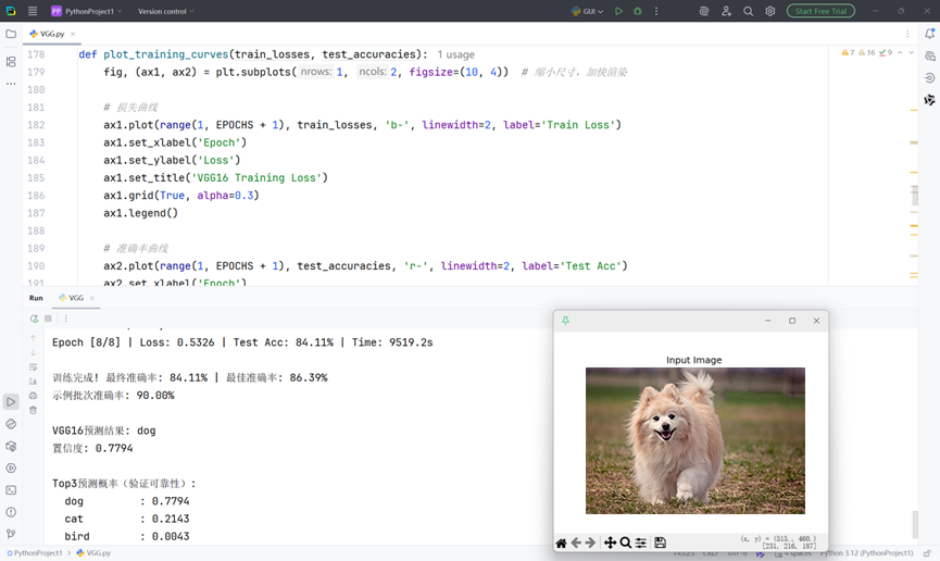
4. 分类结果展示
完整代码
import torch
import torch.nn as nn
import torch.optim as optim
from torchvision import datasets, transforms, models
from torchvision.models import VGG16_Weights
from torch.utils.data import DataLoader
import time
import matplotlib.pyplot as plt
import numpy as np
from PIL import Image
# ---------------------- 1. 核心配置 ----------------------
DEVICE = torch.device("cuda" if torch.cuda.is_available() else "cpu")
BATCH_SIZE = 10  # 平衡内存与速度,CPU无压力
EPOCHS = 8
LEARNING_RATE = 4e-4
NUM_CLASSES = 10
classes = ['airplane', 'automobile', 'bird', 'cat', 'deer',
           'dog', 'frog', 'horse', 'ship', 'truck']
# ---------------------- 2. 数据预处理 ----------------------
cifar_mean = [0.4914, 0.4822, 0.4465]
cifar_std = [0.2023, 0.1994, 0.2010]
transform_train = transforms.Compose([
    transforms.RandomCrop(32, padding=4),  # 保留核心增强(提升泛化,避免识别错误)
    transforms.Resize((144, 144)),  # 核心优化:144×144(速度+准确率平衡点)
    transforms.RandomHorizontalFlip(p=0.5),
    transforms.ToTensor(),
    transforms.Normalize(mean=cifar_mean, std=cifar_std)
])
transform_test = transforms.Compose([
    transforms.Resize((144, 144)),
    transforms.ToTensor(),
    transforms.Normalize(mean=cifar_mean, std=cifar_std)
])
# ---------------------- 3. 数据加载 ----------------------
train_dataset = datasets.CIFAR10(root='./data', train=True, download=True, transform=transform_train)
test_dataset = datasets.CIFAR10(root='./data', train=False, download=True, transform=transform_test)
train_loader = DataLoader(
    train_dataset, batch_size=BATCH_SIZE, shuffle=True,
    num_workers=0, pin_memory=False  # CPU禁用多线程+锁存
)
test_loader = DataLoader(
    test_dataset, batch_size=BATCH_SIZE, shuffle=False,
    num_workers=0, pin_memory=False
)
# ---------------------- 4. 数据集展示 ----------------------
def show_dataset_samples():
    data_iter = iter(train_loader)
    images, labels = next(data_iter)
    fig, axes = plt.subplots(2, 5, figsize=(10, 4))  # 精简布局,减少绘图耗时
    fig.suptitle('CIFAR-10 Dataset Samples (144x144)', fontsize=14, fontweight='bold')
    for i in range(10):
        row, col = i // 5, i % 5
        img = images[i].numpy().transpose((1, 2, 0))
        img = img * cifar_std + cifar_mean
        img = np.clip(img, 0, 1)
        axes[row, col].imshow(img)
        axes[row, col].set_title(classes[labels[i]], fontsize=8)
        axes[row, col].axis('off')
    plt.tight_layout()
    plt.savefig('vgg_dataset_samples_fast.png', dpi=100)  # 降低dpi,加快保存
    plt.show()
print("展示数据集样本...")
show_dataset_samples()
# ---------------------- 5. VGG16模型 ----------------------
model = models.vgg16(weights=VGG16_Weights.IMAGENET1K_V1)
# 优化冻结策略:解冻6层卷积(24-29层),兼顾特征微调与训练速度
for param in model.features[:24].parameters():
    param.requires_grad = False
for param in model.features[24:].parameters():
    param.requires_grad = True
# 保留dropout+适配10分类(防止多轮过拟合)
in_features = model.classifier[6].in_features
model.classifier[6] = nn.Sequential(
    nn.Dropout(0.5),
    nn.Linear(in_features, NUM_CLASSES)
)
model = model.to(DEVICE)
# ---------------------- 6. 优化器 ----------------------
criterion = nn.CrossEntropyLoss()
optimizer = optim.AdamW(
    filter(lambda p: p.requires_grad, model.parameters()),
    lr=LEARNING_RATE, weight_decay=8e-5  # 抑制过拟合
)
# 学习率调度器
scheduler = optim.lr_scheduler.ReduceLROnPlateau(
    optimizer, mode='max', patience=2, factor=0.5
)
# ---------------------- 7. 训练函数 ----------------------
def train_model(model, train_loader, test_loader, criterion, optimizer, scheduler, epochs):
    train_losses = []
    test_accuracies = []
    best_acc = 0.0
    prev_lr = optimizer.param_groups[0]['lr']
    batch_print_interval = 600  # 降低打印频率,减少CPU IO开销
    for epoch in range(epochs):
        start_time = time.time()
        model.train()
        running_loss = 0.0
        # 训练阶段(精简循环,减少冗余计算)
        for batch_idx, (data, targets) in enumerate(train_loader):
            data, targets = data.to(DEVICE), targets.to(DEVICE)
            # 前向+反向传播
            outputs = model(data)
            loss = criterion(outputs, targets)
            optimizer.zero_grad()
            loss.backward()
            optimizer.step()
            running_loss += loss.item() * data.size(0)
            # 批量打印(每600批次一次)
            if batch_idx % batch_print_interval == 0 and batch_idx != 0:
                print(f'  Batch {batch_idx}/{len(train_loader)}, Loss: {loss.item():.4f}')
        # 计算训练损失
        epoch_loss = running_loss / len(train_loader.dataset)
        train_losses.append(epoch_loss)
        # 验证阶段
        model.eval()
        test_correct = 0
        with torch.no_grad():
            for data, targets in test_loader:
                data, targets = data.to(DEVICE), targets.to(DEVICE)
                outputs = model(data)
                _, predicted = torch.max(outputs, 1)
                test_correct += (predicted == targets).sum().item()
        test_acc = 100 * test_correct / len(test_loader.dataset)
        test_accuracies.append(test_acc)
        epoch_time = time.time() - start_time
        # 学习率调度
        scheduler.step(test_acc)
        current_lr = optimizer.param_groups[0]['lr']
        if current_lr != prev_lr:
            print(f'  学习率调整:{prev_lr:.6f} → {current_lr:.6f}')
            prev_lr = current_lr
        # 打印核心信息
        print(
            f'Epoch [{epoch + 1}/{epochs}] | Loss: {epoch_loss:.4f} | Test Acc: {test_acc:.2f}% | Time: {epoch_time:.1f}s')
        # 保存最佳模型(仅最佳时保存,减少IO)
        if test_acc > best_acc:
            best_acc = test_acc
            torch.save(model.state_dict(), "best_vgg16_cifar10_final.pth")
            print(f'  Best model saved! Acc: {best_acc:.2f}%')
    return train_losses, test_accuracies
# ---------------------- 8. 训练曲线可视化 ----------------------
def plot_training_curves(train_losses, test_accuracies):
    fig, (ax1, ax2) = plt.subplots(1, 2, figsize=(10, 4))  # 缩小尺寸,加快渲染
    # 损失曲线
    ax1.plot(range(1, EPOCHS + 1), train_losses, 'b-', linewidth=2, label='Train Loss')
    ax1.set_xlabel('Epoch')
    ax1.set_ylabel('Loss')
    ax1.set_title('VGG16 Training Loss')
    ax1.grid(True, alpha=0.3)
    ax1.legend()
    # 准确率曲线
    ax2.plot(range(1, EPOCHS + 1), test_accuracies, 'r-', linewidth=2, label='Test Acc')
    ax2.set_xlabel('Epoch')
    ax2.set_ylabel('Accuracy (%)')
    ax2.set_title('VGG16 Test Accuracy')
    ax2.grid(True, alpha=0.3)
    ax2.legend()
    plt.suptitle('VGG16 Training History (8 Epochs)', fontsize=14)
    plt.tight_layout()
    plt.savefig('vgg_training_curves_final.png', dpi=100)
    plt.show()
# ---------------------- 9. 分类结果展示(验证识别正确性) ----------------------
def show_classification_results(model, test_loader):
    model.eval()
    images, labels = next(iter(test_loader))
    images = images.to(DEVICE)
    with torch.no_grad():
        outputs = model(images)
        _, predictions = torch.max(outputs, 1)
    fig, axes = plt.subplots(2, 5, figsize=(12, 5))  # 展示10张图,全面验证
    fig.suptitle('VGG16 Classification Results (8 Epochs)', fontsize=14, fontweight='bold')
    for i in range(10):
        row, col = i // 5, i % 5
        img = images[i].cpu().numpy().transpose((1, 2, 0))
        img = img * cifar_std + cifar_mean
        img = np.clip(img, 0, 1)
        true_label = classes[labels[i]]
        pred_label = classes[predictions[i]]
        color = 'green' if true_label == pred_label else 'red'
        axes[row, col].set_title(f'True: {true_label}\nPred: {pred_label}', color=color, fontsize=9)
        axes[row, col].imshow(img)
        axes[row, col].axis('off')
    plt.tight_layout()
    plt.savefig('vgg_classification_results_final.png', dpi=100)
    plt.show()
    # 计算示例批次准确率(验证整体识别效果)
    batch_acc = 100 * (predictions.cpu() == labels).sum().item() / len(labels)
    print(f'示例批次准确率: {batch_acc:.2f}%')
# ---------------------- 10. 主训练流程 ----------------------
if __name__ == "__main__":
    print("=" * 60)
    print(f"VGG16最终训练启动 | Epochs={EPOCHS}, Batch={BATCH_SIZE}, LR={LEARNING_RATE}")
    print(f"训练设备: {DEVICE} | 输入尺寸: 144x144 | 解冻6层卷积")
    print("=" * 60)
    train_losses, test_accuracies = train_model(
        model, train_loader, test_loader, criterion, optimizer, scheduler, EPOCHS
    )
    # 输出核心结果
    final_acc = test_accuracies[-1]
    best_acc = max(test_accuracies)
    print(f"\n训练完成! 最终准确率: {final_acc:.2f}% | 最佳准确率: {best_acc:.2f}%")
    # 核心可视化(验证识别正确性)
    plot_training_curves(train_losses, test_accuracies)
    show_classification_results(model, test_loader)
# ---------------------- 11. 单张图像预测 ----------------------
def predict_single_image(image_path="test_image.jpg"):
    # 构建模型并加载最佳权重
    model = models.vgg16(weights=None)
    in_features = model.classifier[6].in_features
    model.classifier[6] = nn.Sequential(nn.Dropout(0.5), nn.Linear(in_features, NUM_CLASSES))
    model.load_state_dict(torch.load("best_vgg16_cifar10_final.pth", map_location=DEVICE))
    model.to(DEVICE).eval()
    # 预处理匹配144x144输入
    transform = transforms.Compose([
        transforms.Resize((144, 144)),
        transforms.ToTensor(),
        transforms.Normalize(mean=cifar_mean, std=cifar_std)
    ])
    try:
        image = Image.open(image_path).convert("RGB")
        plt.figure(figsize=(5, 5)), plt.imshow(image), plt.axis('off'), plt.title("Input Image"), plt.show()
        with torch.no_grad():
            img_tensor = transform(image).unsqueeze(0).to(DEVICE)
            outputs = model(img_tensor)
            probs = torch.softmax(outputs, dim=1)
            conf, pred = torch.max(probs, 1)
        # 输出详细信息,验证识别正确性
        print(f"\nVGG16预测结果: {classes[pred.item()]}")
        print(f"置信度: {conf.item():.4f}")
        print("\nTop3预测概率(验证可靠性):")
        top3_idx = torch.topk(probs, 3)[1].cpu().numpy()[0]
        for idx in top3_idx:
            print(f"  {classes[idx]:12s}: {probs[0][idx].item():.4f}")
    except FileNotFoundError:
        print(f"错误:未找到图像文件 {image_path}")
# 示例调用(训练完成后执行)
predict_single_image("test_image.jpg")
该模型训练时间较长,可尝试减小输入尺寸、减少解冻卷积层数等提升训练速度。

 浙公网安备 33010602011771号