
7.2.0 头文件
import torch
from torch import nn
from d2l import torch as d2l
from matplotlib import pyplot as plt
7.2.1 定义AlexNet网络模型
# 定义AlexNet网络模型
net = nn.Sequential(
    # 用尺寸更大的11*11卷积窗口来捕捉对象,用更大的步幅来减少输出的高度和宽度
    nn.Conv2d(1, 96, kernel_size=11, stride=4, padding=1),      # 卷积层:输入通道为1,输出通道为96,卷积核尺寸11×11,上下左右填充1层,输出尺寸(1, 96, 54, 54)
    nn.ReLU(),                                                  # 输出尺寸为(1, 96, 54, 54)
    nn.MaxPool2d(kernel_size=3, stride=2),                      # 最大池化层:池化窗口为3×3,步幅为2×2,输出尺寸为(1, 96, 26, 26)
    nn.Conv2d(96, 256, kernel_size=5, padding=2),               # 卷积层,输入通道为96,输出通道为256,卷积核尺寸为5×5,上下左右各填充2层,输出尺寸为(1, 256, 26, 26)
    nn.ReLU(),                                                  # 输出尺寸为(1, 256, 26, 26)
    nn.MaxPool2d(kernel_size=3, stride=2),                      # 最大池化层:池化窗口为3×3,步幅为2×2,输出尺寸为(1, 256, 12, 12)
    nn.Conv2d(256, 384, kernel_size=3, padding=1),              # 卷积层,输入通道为256,输出通道为384,卷积核尺寸为3×3,上下左右各填充1层,输出尺寸为(1, 384, 12, 12)
    nn.ReLU(),                                                  # 输出尺寸为(1, 384, 12, 12)
    nn.Conv2d(384, 384, kernel_size=3, padding=1),              # 卷积层,输入通道为384,输出通道为384,卷积核尺寸为3×3,上下左右各填充1层,输出尺寸为(1, 384, 12, 12)
    nn.ReLU(),                                                  # 输出尺寸为(1, 384, 12, 12)
    nn.Conv2d(384, 256, kernel_size=3, padding=1),              # 卷积层,输入通道为384,输出通道为256,卷积核尺寸为3×3,上下左右各填充1层,输出尺寸为(1, 256, 12, 12)
    nn.ReLU(),                                                  # 输出尺寸为(1, 256, 12, 12)
    nn.MaxPool2d(kernel_size=3, stride=2),                      # 最大池化层:池化窗口为3×3,步幅为2×2,输出尺寸为(1, 256, 5, 5)
    nn.Flatten(),                                               # 输出尺寸为(1, 6400)
    # 用dropout层来减轻过拟合
    nn.Linear(6400, 4096),                                      # 输出尺寸为(1, 4096)
    nn.ReLU(),                                                  # 输出尺寸为(1, 4096)
    nn.Dropout(p=0.5),                                          # 输出尺寸为(1, 4096)
    nn.Linear(4096, 4096),                                      # 输出尺寸为(1, 4096)
    nn.ReLU(),                                                  # 输出尺寸为(1, 4096)
    nn.Dropout(p=0.5),                                          # 输出尺寸为(1, 4096)
    # Fashion-MNIST数据集只有10个类别,所以输出为10
    nn.Linear(4096, 10))                                        # 输出尺寸为(1, 10)

# 定义输入特征X,X的尺寸为(批量大小:1,通道数:1,行数:224,列数:224)
X = torch.randn(1, 1, 224, 224)
for layer in net:
    X=layer(X)
    print(layer.__class__.__name__,'output shape:\t',X.shape)
# 输出:
# Conv2d output shape:     torch.Size([1, 96, 54, 54])
# ReLU output shape:     torch.Size([1, 96, 54, 54])
# MaxPool2d output shape:     torch.Size([1, 96, 26, 26])
# Conv2d output shape:     torch.Size([1, 256, 26, 26])
# ReLU output shape:     torch.Size([1, 256, 26, 26])
# MaxPool2d output shape:     torch.Size([1, 256, 12, 12])
# Conv2d output shape:     torch.Size([1, 384, 12, 12])
# ReLU output shape:     torch.Size([1, 384, 12, 12])
# Conv2d output shape:     torch.Size([1, 384, 12, 12])
# ReLU output shape:     torch.Size([1, 384, 12, 12])
# Conv2d output shape:     torch.Size([1, 256, 12, 12])
# ReLU output shape:     torch.Size([1, 256, 12, 12])
# MaxPool2d output shape:     torch.Size([1, 256, 5, 5])
# Flatten output shape:     torch.Size([1, 6400])
# Linear output shape:     torch.Size([1, 4096])
# ReLU output shape:     torch.Size([1, 4096])
# Dropout output shape:     torch.Size([1, 4096])
# Linear output shape:     torch.Size([1, 4096])
# ReLU output shape:     torch.Size([1, 4096])
# Dropout output shape:     torch.Size([1, 4096])
# Linear output shape:     torch.Size([1, 10])
7.2.2 下载fashion_mnist数据集
# 设置批量大小
batch_size = 128
# 下载fashion_mnist,并对数据集进行打乱和按批量大小进行切割的操作,得到可迭代的训练集和测试集(训练集和测试集的形式都为(特征数据集合,数字标签集合)),同时将图像从28×28放大为224×224
train_iter, test_iter = d2l.load_data_fashion_mnist(batch_size, resize=224)
7.2.3 训练过程
# 定义学习率和训练轮数
lr, num_epochs = 0.01, 10
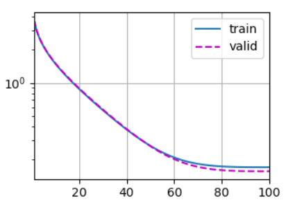
# 使用GPU对模型进行训练,输出最后一轮训练时的平均损失、在训练集上的平均准确率、在测试集上的平均准测率,输出每秒能够训练多少张图像
d2l.train_ch6(net, train_iter, test_iter, num_epochs, lr, d2l.try_gpu())
# loss 0.330, train acc 0.879, test acc 0.884
# 188.7 examples/sec on cuda:0
7.2.4 训练结果可视化
plt.savefig('OutPut.png')
本小节完整代码如下
import torch
from torch import nn
from d2l import torch as d2l
from matplotlib import pyplot as plt

# ------------------------------定义AlexNet网络模型------------------------------------

# 定义AlexNet网络模型
net = nn.Sequential(
    # 用尺寸更大的11*11卷积窗口来捕捉对象,用更大的步幅来减少输出的高度和宽度
    nn.Conv2d(1, 96, kernel_size=11, stride=4, padding=1),      # 卷积层:输入通道为1,输出通道为96,卷积核尺寸11×11,上下左右填充1层,输出尺寸(1, 96, 54, 54)
    nn.ReLU(),                                                  # 输出尺寸为(1, 96, 54, 54)
    nn.MaxPool2d(kernel_size=3, stride=2),                      # 最大池化层:池化窗口为3×3,步幅为2×2,输出尺寸为(1, 96, 26, 26)
    nn.Conv2d(96, 256, kernel_size=5, padding=2),               # 卷积层,输入通道为96,输出通道为256,卷积核尺寸为5×5,上下左右各填充2层,输出尺寸为(1, 256, 26, 26)
    nn.ReLU(),                                                  # 输出尺寸为(1, 256, 26, 26)
    nn.MaxPool2d(kernel_size=3, stride=2),                      # 最大池化层:池化窗口为3×3,步幅为2×2,输出尺寸为(1, 256, 12, 12)
    nn.Conv2d(256, 384, kernel_size=3, padding=1),              # 卷积层,输入通道为256,输出通道为384,卷积核尺寸为3×3,上下左右各填充1层,输出尺寸为(1, 384, 12, 12)
    nn.ReLU(),                                                  # 输出尺寸为(1, 384, 12, 12)
    nn.Conv2d(384, 384, kernel_size=3, padding=1),              # 卷积层,输入通道为384,输出通道为384,卷积核尺寸为3×3,上下左右各填充1层,输出尺寸为(1, 384, 12, 12)
    nn.ReLU(),                                                  # 输出尺寸为(1, 384, 12, 12)
    nn.Conv2d(384, 256, kernel_size=3, padding=1),              # 卷积层,输入通道为384,输出通道为256,卷积核尺寸为3×3,上下左右各填充1层,输出尺寸为(1, 256, 12, 12)
    nn.ReLU(),                                                  # 输出尺寸为(1, 256, 12, 12)
    nn.MaxPool2d(kernel_size=3, stride=2),                      # 最大池化层:池化窗口为3×3,步幅为2×2,输出尺寸为(1, 256, 5, 5)
    nn.Flatten(),                                               # 输出尺寸为(1, 6400)
    # 用dropout层来减轻过拟合
    nn.Linear(6400, 4096),                                      # 输出尺寸为(1, 4096)
    nn.ReLU(),                                                  # 输出尺寸为(1, 4096)
    nn.Dropout(p=0.5),                                          # 输出尺寸为(1, 4096)
    nn.Linear(4096, 4096),                                      # 输出尺寸为(1, 4096)
    nn.ReLU(),                                                  # 输出尺寸为(1, 4096)
    nn.Dropout(p=0.5),                                          # 输出尺寸为(1, 4096)
    # Fashion-MNIST数据集只有10个类别,所以输出为10
    nn.Linear(4096, 10))                                        # 输出尺寸为(1, 10)

# 定义输入特征X,X的尺寸为(批量大小:1,通道数:1,行数:224,列数:224)
X = torch.randn(1, 1, 224, 224)
for layer in net:
    X=layer(X)
    print(layer.__class__.__name__,'output shape:\t',X.shape)
# 输出:
# Conv2d output shape:     torch.Size([1, 96, 54, 54])
# ReLU output shape:     torch.Size([1, 96, 54, 54])
# MaxPool2d output shape:     torch.Size([1, 96, 26, 26])
# Conv2d output shape:     torch.Size([1, 256, 26, 26])
# ReLU output shape:     torch.Size([1, 256, 26, 26])
# MaxPool2d output shape:     torch.Size([1, 256, 12, 12])
# Conv2d output shape:     torch.Size([1, 384, 12, 12])
# ReLU output shape:     torch.Size([1, 384, 12, 12])
# Conv2d output shape:     torch.Size([1, 384, 12, 12])
# ReLU output shape:     torch.Size([1, 384, 12, 12])
# Conv2d output shape:     torch.Size([1, 256, 12, 12])
# ReLU output shape:     torch.Size([1, 256, 12, 12])
# MaxPool2d output shape:     torch.Size([1, 256, 5, 5])
# Flatten output shape:     torch.Size([1, 6400])
# Linear output shape:     torch.Size([1, 4096])
# ReLU output shape:     torch.Size([1, 4096])
# Dropout output shape:     torch.Size([1, 4096])
# Linear output shape:     torch.Size([1, 4096])
# ReLU output shape:     torch.Size([1, 4096])
# Dropout output shape:     torch.Size([1, 4096])
# Linear output shape:     torch.Size([1, 10])

# ------------------------------下载fashion_mnist数据集------------------------------------

# 设置批量大小
batch_size = 128
# 下载fashion_mnist,并对数据集进行打乱和按批量大小进行切割的操作,得到可迭代的训练集和测试集(训练集和测试集的形式都为(特征数据集合,数字标签集合)),同时将图像从28×28放大为224×224
train_iter, test_iter = d2l.load_data_fashion_mnist(batch_size, resize=224)

# ------------------------------训练过程------------------------------------

# 定义学习率和训练轮数
lr, num_epochs = 0.01, 10
# 使用GPU对模型进行训练,输出最后一轮训练时的平均损失、在训练集上的平均准确率、在测试集上的平均准测率,输出每秒能够训练多少张图像
d2l.train_ch6(net, train_iter, test_iter, num_epochs, lr, d2l.try_gpu())
 # loss 0.330, train acc 0.879, test acc 0.884
 # 188.7 examples/sec on cuda:0

# ------------------------------训练结果可视化------------------------------------

plt.savefig('OutPut.png')

 浙公网安备 33010602011771号