《机器学习十讲》第九讲

源地址（相关案例在视频下方）：http://cookdata.cn/auditorium/course_room/10020/

《机器学习十讲》——第九讲（深度学习）

       应用

图像识别：IMAGENET。

机器翻译：Google神经机器翻译系统。

语音识别：

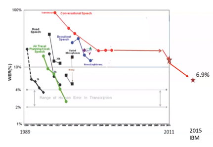
以往GMM-HMM传统方法一直未有突破，2011年使用DNN后获得较大突破，2015年，IBM再次将错误率降低到6.9%，接近人类的平均水平（4%）

游戏：DeepMind团队开发的自我学习玩游戏的系统。

       发展原因

大规模高质量标注数据集出现：IMAGENET

并行运算（如GPU）的发展

更好的非线性激活函数的使用：ReLU代替Logistic

更多优秀的网络结构的发明：ResNet，GoogleNet和AlexNet

深度学习开发平台的发展：TensorFlow，PyTorch和MXNet等

新的正则化技术出现：批标准化，Dropout等

更多稳健的优化算法：SGD的变种：RMSprop，Adam等。

       概念

神经元与感知机：

 

 由输入空间到输出空间的如下函数：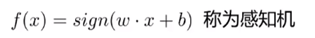

 

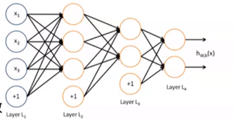
多层感知机（MLP）

定义：多个神经元以全连接层次相连，也称为前馈神经网络。

万能逼近原理：MLP能够逼近任何函数

 

 

 函数逼近：

误差函数：

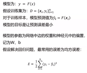
由于深度学习的数据量非常大，所以之前的一些算法不能使用，可以使用随机梯度下降法SGD的一些变种。

梯度计算：后向传播BP

困境：

目标函数通常为非凸函数；极容易陷入局部最优解；随着网络层数增加，容易发生梯度消失或梯度爆炸问题。

机器学习与深度学习的区别：

机器学习需要人工选取特征；深度学习会自动学习有用的特征。

三个·思想：

特征学习（图像识别为例）：深度学习通过层次化的学习方式得到图像特征。

 

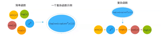
可以将深度学习视为非线性函数逼近器：

深度学习通过一种深层网络结构，实现复杂函数逼近。

万能逼近原理：当隐层节点数目足够多时，具有一个隐层的神经网络，可以以任意精度逼近任意具有有限间断点的函数。

网络层数越多，需要的隐含节点数目指数减小。

 

 

端到端学习：从原始输入直接学习到目标，中间的函数和参数都是可学习。

典型网络结构：

卷积神经网络（VGG / GoogleNet / AlexNet / ResNet）

循环神经网络（RNN）

自编码器（Autoencoder）

生成对抗网络（GAN）

 

卷积神经网络（CNN）：

适合处理网格型数据：物体识别，图片分类，2维网格。

全连接网络不适用于图像：像素大（参数爆炸）

CNN：卷积。（稀疏连接；参数共享；等变表示）

操作：

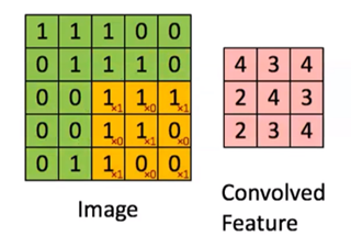
卷积操作：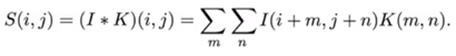

卷积和：

池化

对于局部转换不敏感；在局部节点内进行操作；池化->降采样

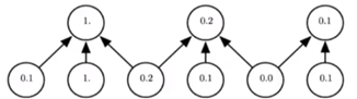
不敏感：图中下方最左0.1改成0.2，0.3不会影响上方1.的变动

最大池化

CNN完整结构：

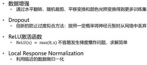
AlexNet：

 

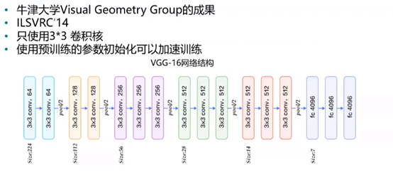
VGG：

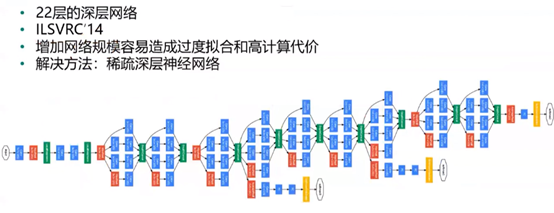
GoogleNet：

ResNet：

RNN：

适合处理训练型数据：自然语言处理等领域。

GAN：

 

 

 　　案例——基于卷积神经网络的人脸识别

#使用sklearn的datasets模块在线获取Olivetti Faces数据集。
from sklearn.datasets import fetch_olivetti_faces
faces = fetch_olivetti_faces()
#打印
faces

 

 该数据集包括四个部分：DESCR主要介绍数据来源；data以一维向量的形式存储了数据集中的400张图像；images以二维矩阵的形式存储了数据集中的400张图像；target存储了数据集中400张图像的类别信息，类别为0-39

#数据结构与类型
print("The shape of data:",faces.data.shape, "The data type of data:",type(faces.data))
print("The shape of images:",faces.images.shape, "The data type of images:",type(faces.images))
print("The shape of target:",faces.target.shape, "The data type of target:",type(faces.target))

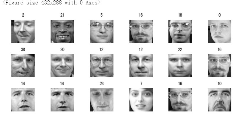
#使用matshow输出部分人脸图片
import numpy as np
rndperm = np.random.permutation(len(faces.images)) #将数据的索引随机打乱
import matplotlib.pyplot as plt
%matplotlib inline
plt.gray()
fig = plt.figure(figsize=(9,4) )
for i in range(0,18):
    ax = fig.add_subplot(3,6,i+1 )
    plt.title(str(faces.target[rndperm[i]])) #类标
    ax.matshow(faces.images[rndperm[i],:]) #图片内容
    plt.box(False) #去掉边框
    plt.axis("off")#不显示坐标轴
plt.tight_layout()  

#查看同一个人的不同人脸特点
labels = [2,11,6] #选取三个人
%matplotlib inline
plt.gray()
fig = plt.figure(figsize=(12,4) )
for i in range(0,3):
    faces_labeli = faces.images[faces.target == labels[i]]
    for j in range(0,10):    
        ax = fig.add_subplot(3,10,10*i + j+1 )
        ax.matshow(faces_labeli[j])
        plt.box(False) #去掉边框
        plt.axis("off")#不显示坐标轴
plt.tight_layout() 

#将数据集划分为训练集和测试集两部分，注意要按照图像标签进行分层采样
# 定义特征和标签
X,y = faces.images,faces.target
# 以5:5比例随机地划分训练集和测试集
from sklearn.model_selection import train_test_split
train_x, test_x, train_y, test_y = train_test_split(X, y, test_size=0.5,stratify = y,random_state=0)
# 记录测试集中出现的类别，后期模型评价画混淆矩阵时需要
#index = set(test_y)

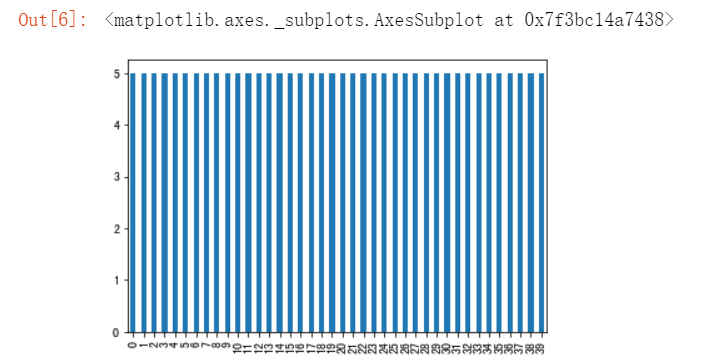
#使用柱状图显示训练集中40人每个人有几张图片
import pandas as pd
pd.Series(train_y).value_counts().sort_index().plot(kind="bar")

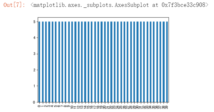
#在测试集中每个人有几张图片
pd.Series(test_y).value_counts().sort_index().plot(kind="bar")

# 转换数据维度，模型训练时要用
train_x = train_x.reshape(train_x.shape[0], 64, 64, 1)
test_x = test_x.reshape(test_x.shape[0], 64, 64, 1)

建立卷积神经网络人脸识别模型——CNN网络结构

#从keras的相应模块引入需要的对象。
import warnings
warnings.filterwarnings('ignore') #该行代码的作用是隐藏警告信息
import tensorflow as tf
import tensorflow.keras.layers as layers
import tensorflow.keras.backend as K
K.clear_session()
#逐层搭建卷积神经网络模型。此处使用了函数式api
inputs = layers.Input(shape=(64,64,1), name='inputs')
conv1 = layers.Conv2D(32,3,3,padding="same",activation="relu",name="conv1")(inputs) #卷积层32
maxpool1 = layers.MaxPool2D(pool_size=(2,2),name="maxpool1")(conv1) #池化层1
conv2 = layers.Conv2D(64,3,3,padding="same",activation="relu",name="conv2")(maxpool1) #卷积层64
maxpool2 = layers.MaxPool2D(pool_size=(2,2),name="maxpool2")(conv2) #池化层2
flatten1 = layers.Flatten(name="flatten1")(maxpool2) #拉成一维
dense1 = layers.Dense(512,activation="tanh",name="dense1")(flatten1)
dense2 = layers.Dense(40,activation="softmax",name="dense2")(dense1) #40个分类
model = tf.keras.Model(inputs,dense2)
#网络结构打印。
model.summary()

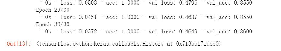
#模型编译，指定误差函数、优化方法和评价指标。使用训练集进行模型训练。
model.compile(loss='sparse_categorical_crossentropy', optimizer="Adam", metrics=['accuracy'])
model.fit(train_x,train_y, batch_size=20, epochs=30, validation_data=(test_x,test_y),verbose=2)

#评价
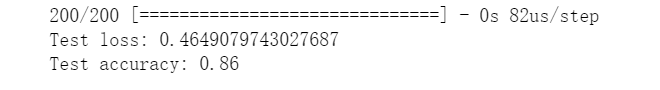
score = model.evaluate(test_x, test_y)
print('Test loss:', score[0])
print('Test accuracy:', score[1])

 

 使用TensorFlow进行数据增强，再进行一次训练

#数据增强——ImageDataGenerator
from tensorflow.keras.preprocessing.image import ImageDataGenerator
# 定义随机变换的类别及程度
datagen = ImageDataGenerator(
        rotation_range=0,            # 图像随机转动的角度
        width_shift_range=0.01,      # 图像水平偏移的幅度
        height_shift_range=0.01,     # 图像竖直偏移的幅度
        shear_range=0.01,            # 逆时针方向的剪切变换角度
        zoom_range=0.01,             # 随机缩放的幅度
        horizontal_flip=True,
        fill_mode='nearest')

#使用增强后的数据进行模型训练与评价
inputs = layers.Input(shape=(64,64,1), name='inputs')
conv1 = layers.Conv2D(32,3,3,padding="same",activation="relu",name="conv1")(inputs)
maxpool1 = layers.MaxPool2D(pool_size=(2,2),name="maxpool1")(conv1)
conv2 = layers.Conv2D(64,3,3,padding="same",activation="relu",name="conv2")(maxpool1)
maxpool2 = layers.MaxPool2D(pool_size=(2,2),name="maxpool2")(conv2)
flatten1 = layers.Flatten(name="flatten1")(maxpool2)
dense1 = layers.Dense(512,activation="tanh",name="dense1")(flatten1)
dense2 = layers.Dense(40,activation="softmax",name="dense2")(dense1)
model2 = tf.keras.Model(inputs,dense2)
model2.compile(loss='sparse_categorical_crossentropy', optimizer="Adam", metrics=['accuracy'])
# 训练模型
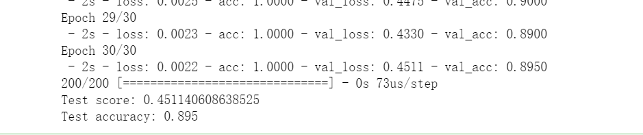
model2.fit_generator(datagen.flow(train_x, train_y, batch_size=200),epochs=30,steps_per_epoch=16, verbose = 2,validation_data=(test_x,test_y))
# 模型评价
score = model2.evaluate(test_x, test_y)
print('Test score:', score[0])
print('Test accuracy:', score[1])