Decision Trees of sklearn

Decision Trees

https://scikit-learn.org/stable/modules/tree.html

    决策树是一种非参数的监督性学习算法， 其跟KNN类似，不依赖参数性模型。

   可以用于分类和回归。

   从特征中学习出决策规则。

Decision Trees (DTs) are a non-parametric supervised learning method used for classification and regression. The goal is to create a model that predicts the value of a target variable by learning simple decision rules inferred from the data features. A tree can be seen as a piecewise constant approximation.

For instance, in the example below, decision trees learn from data to approximate a sine curve with a set of if-then-else decision rules. The deeper the tree, the more complex the decision rules and the fitter the model.

 

优点：

简单易懂和可视化

需要较少的数据准备

算法具有log级别的时间复杂度

处理数值型和分类型数据

多输出支持

 

Some advantages of decision trees are:

• Simple to understand and to interpret. Trees can be visualised.

• Requires little data preparation. Other techniques often require data normalisation, dummy variables need to be created and blank values to be removed. Note however that this module does not support missing values.

• The cost of using the tree (i.e., predicting data) is logarithmic in the number of data points used to train the tree.

• Able to handle both numerical and categorical data. However scikit-learn implementation does not support categorical variables for now. Other techniques are usually specialised in analysing datasets that have only one type of variable. See algorithms for more information.

• Able to handle multi-output problems.

• Uses a white box model. If a given situation is observable in a model, the explanation for the condition is easily explained by boolean logic. By contrast, in a black box model (e.g., in an artificial neural network), results may be more difficult to interpret.

• Possible to validate a model using statistical tests. That makes it possible to account for the reliability of the model.

• Performs well even if its assumptions are somewhat violated by the true model from which the data were generated.

缺点：

容易过拟合

对于数据敏感，不稳定

预测不平滑和连续

The disadvantages of decision trees include:

• Decision-tree learners can create over-complex trees that do not generalise the data well. This is called overfitting. Mechanisms such as pruning, setting the minimum number of samples required at a leaf node or setting the maximum depth of the tree are necessary to avoid this problem.

• Decision trees can be unstable because small variations in the data might result in a completely different tree being generated. This problem is mitigated by using decision trees within an ensemble.

• Predictions of decision trees are neither smooth nor continuous, but piecewise constant approximations as seen in the above figure. Therefore, they are not good at extrapolation.

• The problem of learning an optimal decision tree is known to be NP-complete under several aspects of optimality and even for simple concepts. Consequently, practical decision-tree learning algorithms are based on heuristic algorithms such as the greedy algorithm where locally optimal decisions are made at each node. Such algorithms cannot guarantee to return the globally optimal decision tree. This can be mitigated by training multiple trees in an ensemble learner, where the features and samples are randomly sampled with replacement.

• There are concepts that are hard to learn because decision trees do not express them easily, such as XOR, parity or multiplexer problems.

• Decision tree learners create biased trees if some classes dominate. It is therefore recommended to balance the dataset prior to fitting with the decision tree.

 

Classification

应用于分类，支持多类分类。

DecisionTreeClassifier is a class capable of performing multi-class classification on a dataset.

As with other classifiers, DecisionTreeClassifier takes as input two arrays: an array X, sparse or dense, of shape (n_samples, n_features) holding the training samples, and an array Y of integer values, shape (n_samples,), holding the class labels for the training samples:

from sklearn import tree
X = [[0, 0], [1, 1]]
Y = [0, 1]
clf = tree.DecisionTreeClassifier()
clf = clf.fit(X, Y)

After being fitted, the model can then be used to predict the class of samples:

>>> clf.predict([[2., 2.]])
array([1])

支持二值分类和多类分类。

DecisionTreeClassifier is capable of both binary (where the labels are [-1, 1]) classification and multiclass (where the labels are [0, …, K-1]) classification.

Using the Iris dataset, we can construct a tree as follows:

from sklearn.datasets import load_iris
from sklearn import tree
X, y = load_iris(return_X_y=True)
clf = tree.DecisionTreeClassifier()
clf = clf.fit(X, y)

Once trained, you can plot the tree with the plot_tree function:

打印决策树图

tree.plot_tree(clf) 

 

 

 

打印文本形式的树

Alternatively, the tree can also be exported in textual format with the function export_text. This method doesn’t require the installation of external libraries and is more compact:

>>> from sklearn.datasets import load_iris
>>> from sklearn.tree import DecisionTreeClassifier
>>> from sklearn.tree import export_text
>>> iris = load_iris()
>>> decision_tree = DecisionTreeClassifier(random_state=0, max_depth=2)
>>> decision_tree = decision_tree.fit(iris.data, iris.target)
>>> r = export_text(decision_tree, feature_names=iris['feature_names'])
>>> print(r)
|--- petal width (cm) <= 0.80
|   |--- class: 0
|--- petal width (cm) >  0.80
|   |--- petal width (cm) <= 1.75
|   |   |--- class: 1
|   |--- petal width (cm) >  1.75
|   |   |--- class: 2

 

DecisionTreeClassifier

https://scikit-learn.org/stable/modules/generated/sklearn.tree.DecisionTreeClassifier.html#sklearn.tree.DecisionTreeClassifier

 

>>> from sklearn.datasets import load_iris
>>> from sklearn.model_selection import cross_val_score
>>> from sklearn.tree import DecisionTreeClassifier
>>> clf = DecisionTreeClassifier(random_state=0)
>>> iris = load_iris()
>>> cross_val_score(clf, iris.data, iris.target, cv=10)
...                             
...
array([ 1.     ,  0.93...,  0.86...,  0.93...,  0.93...,
        0.93...,  0.93...,  1.     ,  0.93...,  1.      ])

 

 

Plot the decision surface of a decision tree on the iris dataset -- 示例

https://scikit-learn.org/stable/auto_examples/tree/plot_iris_dtc.html#sphx-glr-auto-examples-tree-plot-iris-dtc-py

      决策树应用于两个iris特征， 并使用contur图打印决策线。

     后应用于四个特征，打印树图。

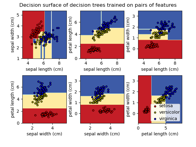
Plot the decision surface of a decision tree trained on pairs of features of the iris dataset.

See decision tree for more information on the estimator.

For each pair of iris features, the decision tree learns decision boundaries made of combinations of simple thresholding rules inferred from the training samples.

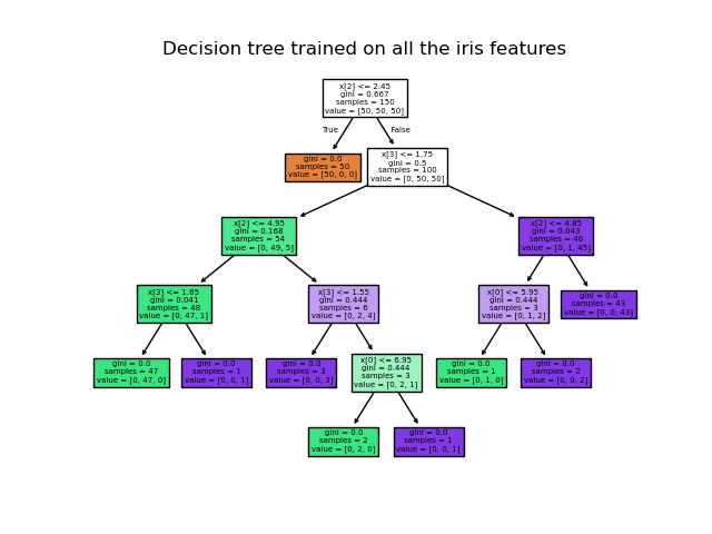
We also show the tree structure of a model built on all of the features.

• 
• 

 

print(__doc__)

import numpy as np
import matplotlib.pyplot as plt

from sklearn.datasets import load_iris
from sklearn.tree import DecisionTreeClassifier, plot_tree

# Parameters
n_classes = 3
plot_colors = "ryb"
plot_step = 0.02

# Load data
iris = load_iris()

for pairidx, pair in enumerate([[0, 1], [0, 2], [0, 3],
                                [1, 2], [1, 3], [2, 3]]):
    # We only take the two corresponding features
    X = iris.data[:, pair]
    y = iris.target

    # Train
    clf = DecisionTreeClassifier().fit(X, y)

    # Plot the decision boundary
    plt.subplot(2, 3, pairidx + 1)

    x_min, x_max = X[:, 0].min() - 1, X[:, 0].max() + 1
    y_min, y_max = X[:, 1].min() - 1, X[:, 1].max() + 1
    xx, yy = np.meshgrid(np.arange(x_min, x_max, plot_step),
                         np.arange(y_min, y_max, plot_step))
    plt.tight_layout(h_pad=0.5, w_pad=0.5, pad=2.5)

    Z = clf.predict(np.c_[xx.ravel(), yy.ravel()])
    Z = Z.reshape(xx.shape)
    cs = plt.contourf(xx, yy, Z, cmap=plt.cm.RdYlBu)

    plt.xlabel(iris.feature_names[pair[0]])
    plt.ylabel(iris.feature_names[pair[1]])

    # Plot the training points
    for i, color in zip(range(n_classes), plot_colors):
        idx = np.where(y == i)
        plt.scatter(X[idx, 0], X[idx, 1], c=color, label=iris.target_names[i],
                    cmap=plt.cm.RdYlBu, edgecolor='black', s=15)

plt.suptitle("Decision surface of a decision tree using paired features")
plt.legend(loc='lower right', borderpad=0, handletextpad=0)
plt.axis("tight")

plt.figure()
clf = DecisionTreeClassifier().fit(iris.data, iris.target)
plot_tree(clf, filled=True)
plt.show()

 

Understanding the decision tree structure -- 示例

https://scikit-learn.org/stable/auto_examples/tree/plot_unveil_tree_structure.html#sphx-glr-auto-examples-tree-plot-unveil-tree-structure-py

探索决策树内部数据结构。

The decision tree structure can be analysed to gain further insight on the relation between the features and the target to predict. In this example, we show how to retrieve:

• the binary tree structure;

• the depth of each node and whether or not it’s a leaf;

• the nodes that were reached by a sample using the decision_path method;

• the leaf that was reached by a sample using the apply method;

• the rules that were used to predict a sample;

• the decision path shared by a group of samples.

 

Regression

决策树应用于回归。

Decision trees can also be applied to regression problems, using the DecisionTreeRegressor class.

As in the classification setting, the fit method will take as argument arrays X and y, only that in this case y is expected to have floating point values instead of integer values:

 

>>> from sklearn import tree
>>> X = [[0, 0], [2, 2]]
>>> y = [0.5, 2.5]
>>> clf = tree.DecisionTreeRegressor()
>>> clf = clf.fit(X, y)
>>> clf.predict([[1, 1]])
array([0.5])

 

DecisionTreeRegressor

https://scikit-learn.org/stable/modules/generated/sklearn.tree.DecisionTreeRegressor.html#sklearn.tree.DecisionTreeRegressor

 

>>> from sklearn.datasets import load_diabetes
>>> from sklearn.model_selection import cross_val_score
>>> from sklearn.tree import DecisionTreeRegressor
>>> X, y = load_diabetes(return_X_y=True)
>>> regressor = DecisionTreeRegressor(random_state=0)
>>> cross_val_score(regressor, X, y, cv=10)
...                    
...
array([-0.39..., -0.46...,  0.02...,  0.06..., -0.50...,
       0.16...,  0.11..., -0.73..., -0.30..., -0.00...])

 

Decision Tree Regression

https://scikit-learn.org/stable/auto_examples/tree/plot_tree_regression.html#sphx-glr-auto-examples-tree-plot-tree-regression-py

    一维度回归。

    决策树应用于添加噪音的sin曲线。

    max_depth 越大越会产生过拟合。

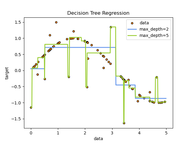
A 1D regression with decision tree.

The decision trees is used to fit a sine curve with addition noisy observation. As a result, it learns local linear regressions approximating the sine curve.

We can see that if the maximum depth of the tree (controlled by the max_depth parameter) is set too high, the decision trees learn too fine details of the training data and learn from the noise, i.e. they overfit.

 

print(__doc__)

# Import the necessary modules and libraries
import numpy as np
from sklearn.tree import DecisionTreeRegressor
import matplotlib.pyplot as plt

# Create a random dataset
rng = np.random.RandomState(1)
X = np.sort(5 * rng.rand(80, 1), axis=0)
y = np.sin(X).ravel()
y[::5] += 3 * (0.5 - rng.rand(16))

# Fit regression model
regr_1 = DecisionTreeRegressor(max_depth=2)
regr_2 = DecisionTreeRegressor(max_depth=5)
regr_1.fit(X, y)
regr_2.fit(X, y)

# Predict
X_test = np.arange(0.0, 5.0, 0.01)[:, np.newaxis]
y_1 = regr_1.predict(X_test)
y_2 = regr_2.predict(X_test)

# Plot the results
plt.figure()
plt.scatter(X, y, s=20, edgecolor="black",
            c="darkorange", label="data")
plt.plot(X_test, y_1, color="cornflowerblue",
         label="max_depth=2", linewidth=2)
plt.plot(X_test, y_2, color="yellowgreen", label="max_depth=5", linewidth=2)
plt.xlabel("data")
plt.ylabel("target")
plt.title("Decision Tree Regression")
plt.legend()
plt.show()

 

Multi-output problems

决策树支持多目标分类

如果多个目标是独立的，对于每一个目标使用独立的模型，进行训练预测。

但是往往目标之间是依赖的， 所以使用支持多目标的模型，具有优点：

（1）由于学习到目标之间的依赖关系， 那么预测的精度有提升

（2）只需要单个模型学习， 训练速度有提升

A multi-output problem is a supervised learning problem with several outputs to predict, that is when Y is a 2d array of shape (n_samples, n_outputs).

When there is no correlation between the outputs, a very simple way to solve this kind of problem is to build n independent models, i.e. one for each output, and then to use those models to independently predict each one of the n outputs. However, because it is likely that the output values related to the same input are themselves correlated, an often better way is to build a single model capable of predicting simultaneously all n outputs. First, it requires lower training time since only a single estimator is built. Second, the generalization accuracy of the resulting estimator may often be increased.

With regard to decision trees, this strategy can readily be used to support multi-output problems. This requires the following changes:

• Store n output values in leaves, instead of 1;

• Use splitting criteria that compute the average reduction across all n outputs.

This module offers support for multi-output problems by implementing this strategy in both DecisionTreeClassifier and DecisionTreeRegressor. If a decision tree is fit on an output array Y of shape (n_samples, n_outputs) then the resulting estimator will:

• Output n_output values upon predict;

• Output a list of n_output arrays of class probabilities upon predict_proba.

The use of multi-output trees for regression is demonstrated in Multi-output Decision Tree Regression. In this example, the input X is a single real value and the outputs Y are the sine and cosine of X.

 

Multi-output Decision Tree Regression -- 示例

https://scikit-learn.org/stable/auto_examples/tree/plot_tree_regression_multioutput.html#sphx-glr-auto-examples-tree-plot-tree-regression-multioutput-py

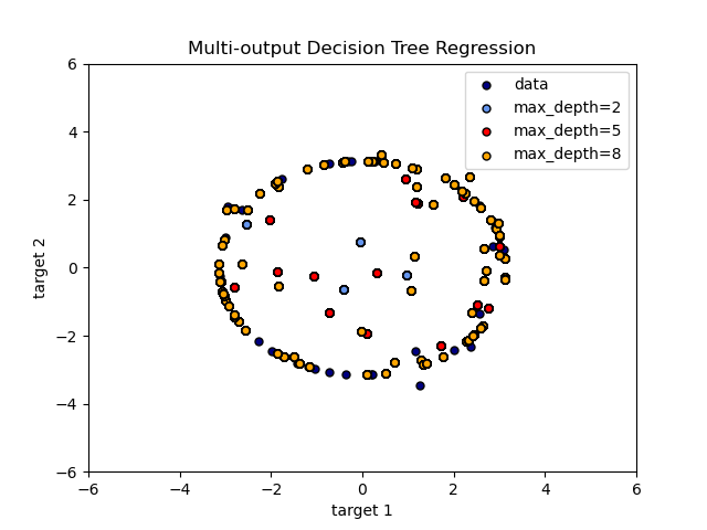
   构造sine和cos多值目标， 打印此二维目标 和 预测结果。

An example to illustrate multi-output regression with decision tree.

The decision trees is used to predict simultaneously the noisy x and y observations of a circle given a single underlying feature. As a result, it learns local linear regressions approximating the circle.

We can see that if the maximum depth of the tree (controlled by the max_depth parameter) is set too high, the decision trees learn too fine details of the training data and learn from the noise, i.e. they overfit.

 

print(__doc__)

import numpy as np
import matplotlib.pyplot as plt
from sklearn.tree import DecisionTreeRegressor

# Create a random dataset
rng = np.random.RandomState(1)
X = np.sort(200 * rng.rand(100, 1) - 100, axis=0)
y = np.array([np.pi * np.sin(X).ravel(), np.pi * np.cos(X).ravel()]).T
y[::5, :] += (0.5 - rng.rand(20, 2))

# Fit regression model
regr_1 = DecisionTreeRegressor(max_depth=2)
regr_2 = DecisionTreeRegressor(max_depth=5)
regr_3 = DecisionTreeRegressor(max_depth=8)
regr_1.fit(X, y)
regr_2.fit(X, y)
regr_3.fit(X, y)

# Predict
X_test = np.arange(-100.0, 100.0, 0.01)[:, np.newaxis]
y_1 = regr_1.predict(X_test)
y_2 = regr_2.predict(X_test)
y_3 = regr_3.predict(X_test)

# Plot the results
plt.figure()
s = 25
plt.scatter(y[:, 0], y[:, 1], c="navy", s=s,
            edgecolor="black", label="data")
plt.scatter(y_1[:, 0], y_1[:, 1], c="cornflowerblue", s=s,
            edgecolor="black", label="max_depth=2")
plt.scatter(y_2[:, 0], y_2[:, 1], c="red", s=s,
            edgecolor="black", label="max_depth=5")
plt.scatter(y_3[:, 0], y_3[:, 1], c="orange", s=s,
            edgecolor="black", label="max_depth=8")
plt.xlim([-6, 6])
plt.ylim([-6, 6])
plt.xlabel("target 1")
plt.ylabel("target 2")
plt.title("Multi-output Decision Tree Regression")
plt.legend(loc="best")
plt.show()

 

Tips on practical use

 特征数目太多，同时样本太少，容易导致过拟合

考虑特征维度约减（使用 PCA 特征选择）

可视化是个展示的好工具

样本的数量必须二倍于输的深度

树林的集成学习，可消减拟合。

• Decision trees tend to overfit on data with a large number of features. Getting the right ratio of samples to number of features is important, since a tree with few samples in high dimensional space is very likely to overfit.

• Consider performing dimensionality reduction (PCA, ICA, or Feature selection) beforehand to give your tree a better chance of finding features that are discriminative.

• Understanding the decision tree structure will help in gaining more insights about how the decision tree makes predictions, which is important for understanding the important features in the data.

• Visualise your tree as you are training by using the export function. Use max_depth=3 as an initial tree depth to get a feel for how the tree is fitting to your data, and then increase the depth.

• Remember that the number of samples required to populate the tree doubles for each additional level the tree grows to. Use max_depth to control the size of the tree to prevent overfitting.

• Use min_samples_split or min_samples_leaf to ensure that multiple samples inform every decision in the tree, by controlling which splits will be considered. A very small number will usually mean the tree will overfit, whereas a large number will prevent the tree from learning the data. Try min_samples_leaf=5 as an initial value. If the sample size varies greatly, a float number can be used as percentage in these two parameters. While min_samples_split can create arbitrarily small leaves, min_samples_leaf guarantees that each leaf has a minimum size, avoiding low-variance, over-fit leaf nodes in regression problems. For classification with few classes, min_samples_leaf=1 is often the best choice.

  Note that min_samples_split considers samples directly and independent of sample_weight, if provided (e.g. a node with m weighted samples is still treated as having exactly m samples). Consider min_weight_fraction_leaf or min_impurity_decrease if accounting for sample weights is required at splits.

• Balance your dataset before training to prevent the tree from being biased toward the classes that are dominant. Class balancing can be done by sampling an equal number of samples from each class, or preferably by normalizing the sum of the sample weights (sample_weight) for each class to the same value. Also note that weight-based pre-pruning criteria, such as min_weight_fraction_leaf, will then be less biased toward dominant classes than criteria that are not aware of the sample weights, like min_samples_leaf.

• If the samples are weighted, it will be easier to optimize the tree structure using weight-based pre-pruning criterion such as min_weight_fraction_leaf, which ensure that leaf nodes contain at least a fraction of the overall sum of the sample weights.

• All decision trees use np.float32 arrays internally. If training data is not in this format, a copy of the dataset will be made.

• If the input matrix X is very sparse, it is recommended to convert to sparse csc_matrix before calling fit and sparse csr_matrix before calling predict. Training time can be orders of magnitude faster for a sparse matrix input compared to a dense matrix when features have zero values in most of the samples.

 

https://paradiseeee.github.io/2019/02/28/Python-DataScience-CookBook-Learning-Notes-(II)/

• 关于决策树的基础知识参考“R 统计学习笔记”
• 一些提高效率，短时间生成较合理的决策树的算法：
  • Hunt
  • ID3
  • C4.5
  • CART
• target 的属性种类：
  • 二元属性
  • 标称属性（n 个值）
  • 序数属性（如：小中大）
  • 连续属性（连续变量离散化形成）
• 决策树的不足：
  • 容易过拟合
  • 给定一个数据集，能产生巨量的决策树
  • 对类别不平衡敏感