matplotlib subplot 子图

总括

MATLAB和pyplot有当前的图形（figure）和当前的轴（axes）的概念，所有的作图命令都是对当前的对象作用。可以通过gca()获得当前的axes（轴），通过gcf()获得当前的图形（figure）

import numpy as np
import matplotlib.pyplot as plt
def f(t):
return np.exp(-t) * np.cos(2*np.pi*t)
t1 = np.arange(0.0, 5.0, 0.1)
t2 = np.arange(0.0, 5.0, 0.02)
plt.figure(1)
plt.subplot(211)
plt.plot(t1, f(t1), 'bo', t2, f(t2), 'k')
plt.subplot(212)
plt.plot(t2, np.cos(2*np.pi*t2), 'r--')
plt.show()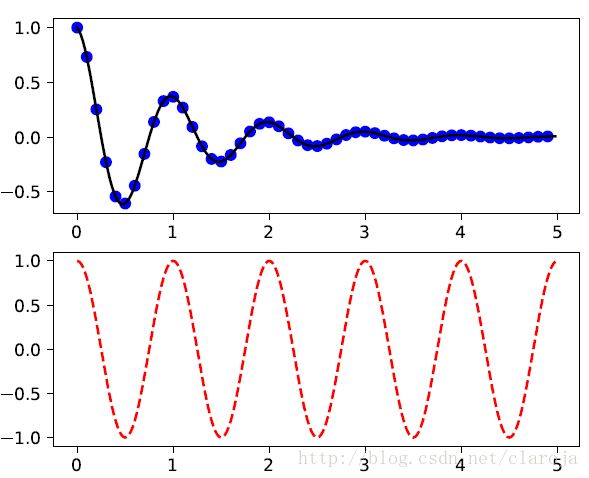

 
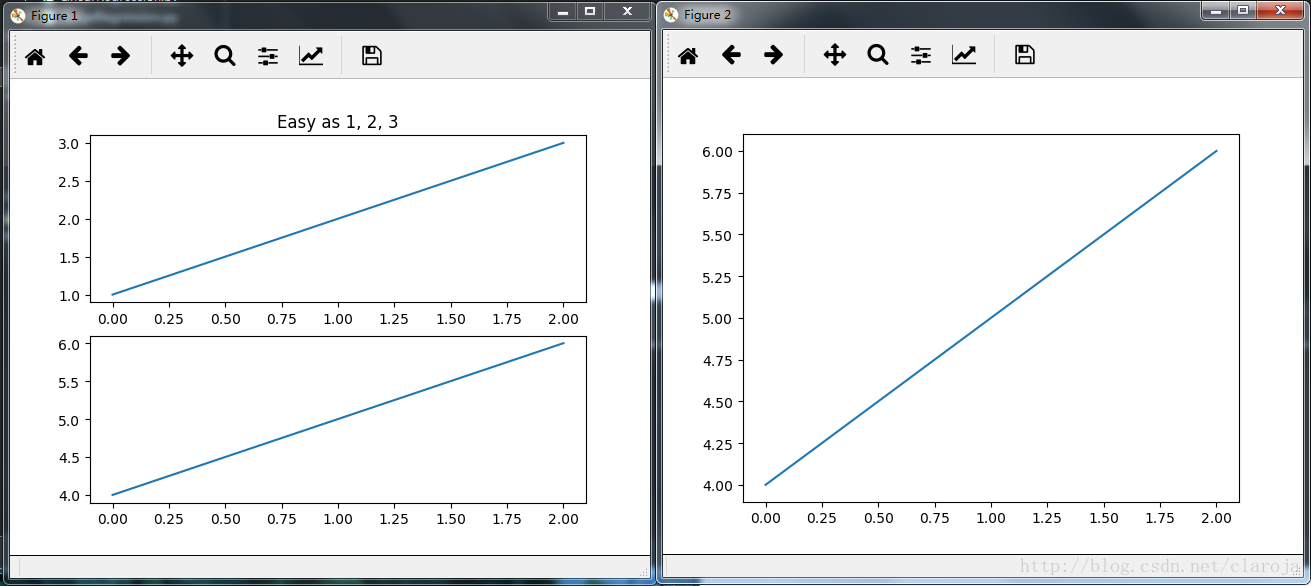
如果不指定figure()的轴，figure(1)命令默认会被建立，同样的如果你不指定subplot(numrows, numcols, fignum)的轴，subplot(111)也会自动建立。

import matplotlib.pyplot as plt
plt.figure(1) # 创建第一个画板（figure）
plt.subplot(211) # 第一个画板的第一个子图
plt.plot([1, 2, 3])
plt.subplot(212) # 第二个画板的第二个子图
plt.plot([4, 5, 6])
plt.figure(2) #创建第二个画板
plt.plot([4, 5, 6]) # 默认子图命令是subplot(111)
plt.figure(1) # 调取画板1; subplot(212)仍然被调用中
plt.subplot(211) #调用subplot(211)
plt.title('Easy as 1, 2, 3') # 做出211的标题

subplot()是将整个figure均等分割，而axes()则可以在figure上画图。

import matplotlib.pyplot as plt
import numpy as np
# 创建数据
dt = 0.001
t = np.arange(0.0, 10.0, dt)
r = np.exp(-t[:1000]/0.05) # impulse response
x = np.random.randn(len(t))
s = np.convolve(x, r)[:len(x)]*dt # colored noise
# 默认主轴图axes是subplot(111)
plt.plot(t, s)
plt.axis([0, 1, 1.1*np.amin(s), 2*np.amax(s)])
plt.xlabel('time (s)')
plt.ylabel('current (nA)')
plt.title('Gaussian colored noise')
#内嵌图
a = plt.axes([.65, .6, .2, .2], facecolor='y')
n, bins, patches = plt.hist(s, 400, normed=1)
plt.title('Probability')
plt.xticks([])
plt.yticks([])
#另外一个内嵌图
a = plt.axes([0.2, 0.6, .2, .2], facecolor='y')
plt.plot(t[:len(r)], r)
plt.title('Impulse response')
plt.xlim(0, 0.2)
plt.xticks([])
plt.yticks([])
plt.show()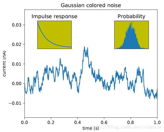

你可以通过clf()清空当前的图板（figure），通过cla()来清理当前的轴（axes）。你需要特别注意的是记得使用close()关闭当前figure画板

通过GridSpec来定制Subplot的坐标

GridSpec指定子图所放置的几何网格。 
SubplotSpec在GridSpec中指定子图（subplot）的位置。 
subplot2grid类似于“pyplot.subplot”，但是它从0开始索引

ax = plt.subplot2grid((2,2),(0, 0))
ax = plt.subplot(2,2,1)

以上两行的子图（subplot）命令是相同的。subplot2grid使用的命令类似于HTML语言。

ax1 = plt.subplot2grid((3,3), (0,0), colspan=3)
ax2 = plt.subplot2grid((3,3), (1,0), colspan=2)
ax3 = plt.subplot2grid((3,3), (1, 2), rowspan=2)
ax4 = plt.subplot2grid((3,3), (2, 0))
ax5 = plt.subplot2grid((3,3), (2, 1))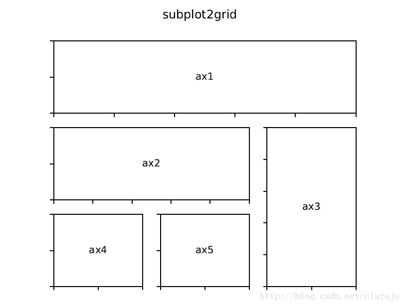

使用GridSpec 和 SubplotSpec

ax = plt.subplot2grid((2,2),(0, 0))

 

相当于

import matplotlib.gridspec as gridspec
gs = gridspec.GridSpec(2, 2)
ax = plt.subplot(gs[0, 0])

一个gridspec实例提供给了类似数组的索引来返回SubplotSpec实例，所以我们可以使用切片（slice）来合并单元格。

gs = gridspec.GridSpec(3, 3)
ax1 = plt.subplot(gs[0, :])
ax2 = plt.subplot(gs[1,:-1])
ax3 = plt.subplot(gs[1:, -1])
ax4 = plt.subplot(gs[-1,0])
ax5 = plt.subplot(gs[-1,-2])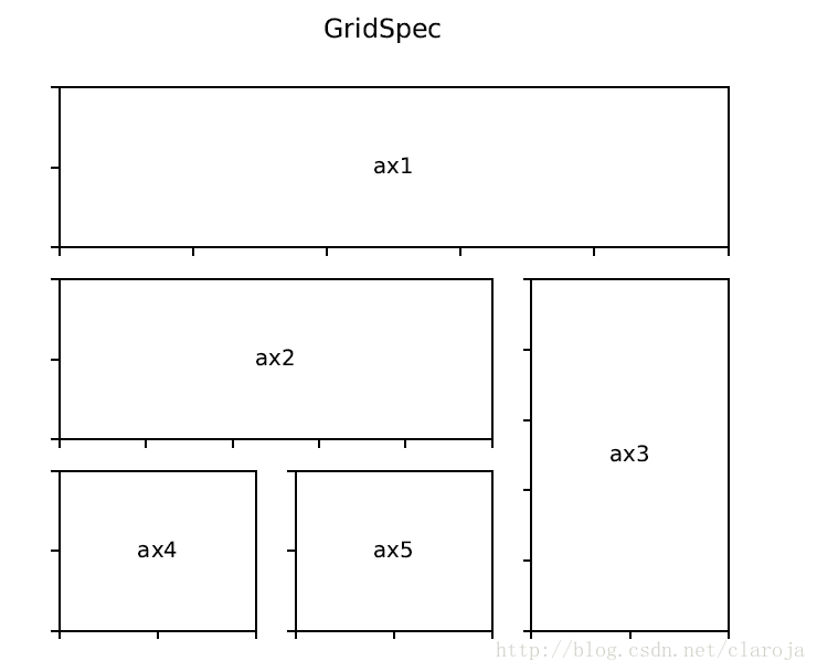

调整GridSpec图层

当GridSpec被使用后，你可以调整子图（subplot）的参数。这个类似于subplot_adjust，但是它只作用于GridSpec实例。

gs1 = gridspec.GridSpec(3, 3)
gs1.update(left=0.05, right=0.48, wspace=0.05)
ax1 = plt.subplot(gs1[:-1, :])
ax2 = plt.subplot(gs1[-1, :-1])
ax3 = plt.subplot(gs1[-1, -1])
gs2 = gridspec.GridSpec(3, 3)
gs2.update(left=0.55, right=0.98, hspace=0.05)
ax4 = plt.subplot(gs2[:, :-1])
ax5 = plt.subplot(gs2[:-1, -1])
ax6 = plt.subplot(gs2[-1, -1])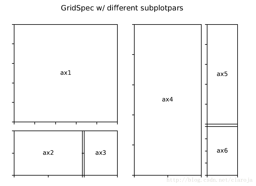

在subplotSpec中嵌套GridSpec

gs0 = gridspec.GridSpec(1, 2)
gs00 = gridspec.GridSpecFromSubplotSpec(3, 3, subplot_spec=gs0[0])
gs01 = gridspec.GridSpecFromSubplotSpec(3, 3, subplot_spec=gs0[1])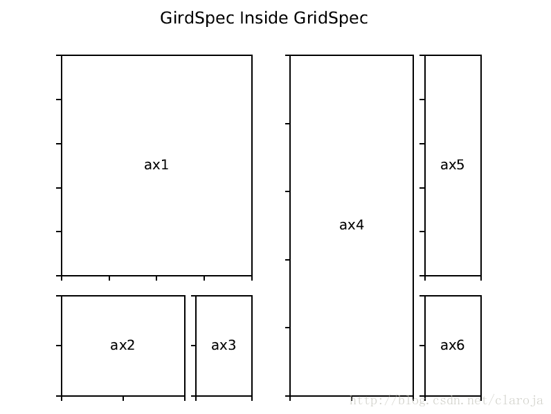

 
下图是一个3*3方格，嵌套在4*4方格中的例子 
 
调整GridSpec的尺寸 
默认的，GridSpec会创建相同尺寸的单元格。你可以调整相关的行与列的高度和宽度。注意，绝对值是不起作用的，相对值才起作用。

gs = gridspec.GridSpec(2, 2,
                        width_ratios=[1,2],
                        height_ratios=[4,1]
                        )
ax1 = plt.subplot(gs[0])
ax2 = plt.subplot(gs[1])
ax3 = plt.subplot(gs[2])
ax4 = plt.subplot(gs[3])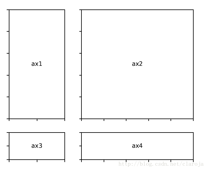

调整图层

tigh_layout自动调整子图（subplot）参数来适应画板（figure）的区域。它只会检查刻度标签（ticklabel），坐标轴标签（axis label），标题（title）。 
轴（axes）包括子图（subplot）被画板（figure）的坐标指定。所以一些标签会超越画板（figure）的范围。

plt.rcParams['savefig.facecolor'] = "0.8"
def example_plot(ax, fontsize=12):
    ax.plot([1, 2])
    ax.locator_params(nbins=3)
    ax.set_xlabel('x-label', fontsize=fontsize)
    ax.set_ylabel('y-label', fontsize=fontsize)
    ax.set_title('Title', fontsize=fontsize)
plt.close('all')
fig, ax = plt.subplots()
example_plot(ax, fontsize=24)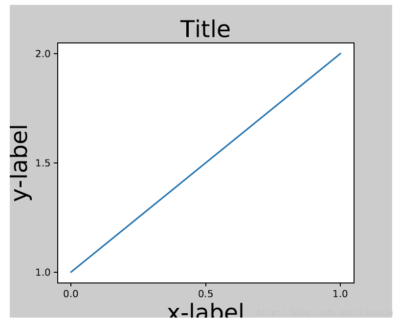

 
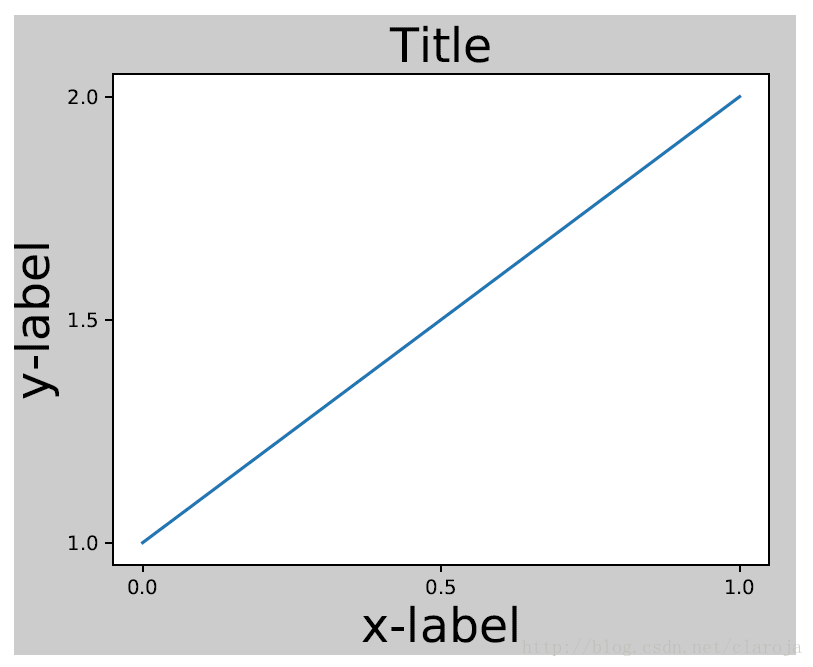
对于子图（subplot）可以通过调整subplot参数解决这个问题。Matplotlib v1.1 引进了一个新的命令tight_layout()自动的解决这个问题

plt.tight_layout()

 

 
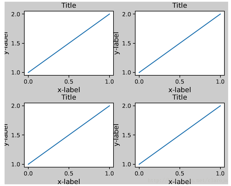
很多子图的情况

plt.close('all')
fig, ((ax1, ax2), (ax3, ax4)) = plt.subplots(nrows=2, ncols=2)
example_plot(ax1)
example_plot(ax2)
example_plot(ax3)
example_plot(ax4)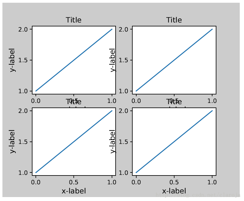

plt.tight_layout()

 

 
tight_layout()含有pad，w_pad和h_pad

plt.tight_layout(pad=0.4, w_pad=0.5, h_pad=1.0)

 

在GridSpec中使用tight_layout()

GridSpec拥有它自己的tight_layout()方法

plt.close('all')
fig = plt.figure()
import matplotlib.gridspec as gridspec
gs1 = gridspec.GridSpec(2, 1)
ax1 = fig.add_subplot(gs1[0])
ax2 = fig.add_subplot(gs1[1])
example_plot(ax1)
example_plot(ax2)
gs1.tight_layout(fig)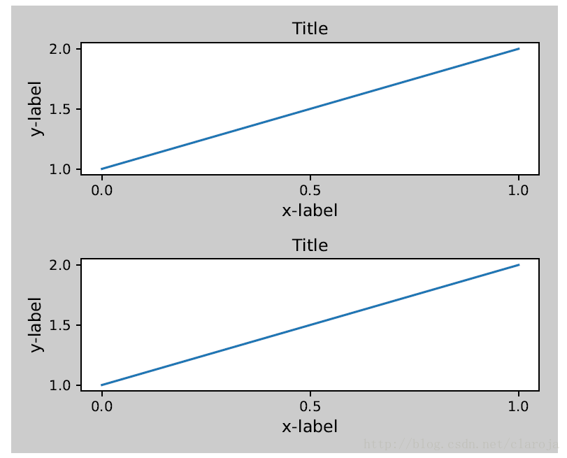

 
你可以指定一个可选择的方形（rect）参数来指定子图（subplot）到画板（figure）的距离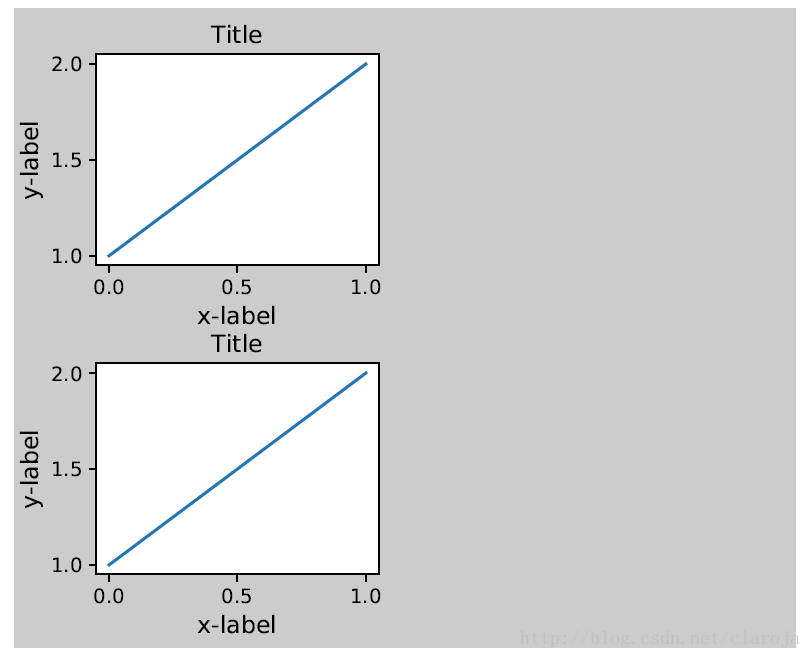 
 
这个还可以应用到复合的gridspecs中

gs2 = gridspec.GridSpec(3, 1)
for ss in gs2:
ax = fig.add_subplot(ss)
example_plot(ax)
ax.set_title("")
ax.set_xlabel("")
ax.set_xlabel("x-label", fontsize=12)
gs2.tight_layout(fig, rect=[0.5, 0, 1, 1], h_pad=0.5)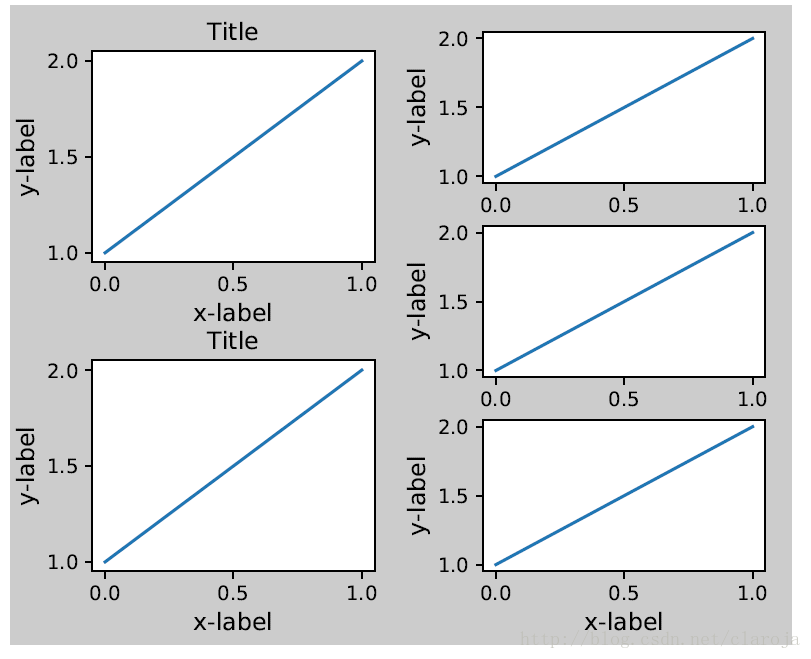

在AxesGrid1中使用tight_layout()

plt.close('all')
fig = plt.figure()
from mpl_toolkits.axes_grid1 import Grid
grid = Grid(fig, rect=111, nrows_ncols=(2,2),
axes_pad=0.25, label_mode='L',
)
for ax in grid:
example_plot(ax)
ax.title.set_visible(False)
plt.tight_layout()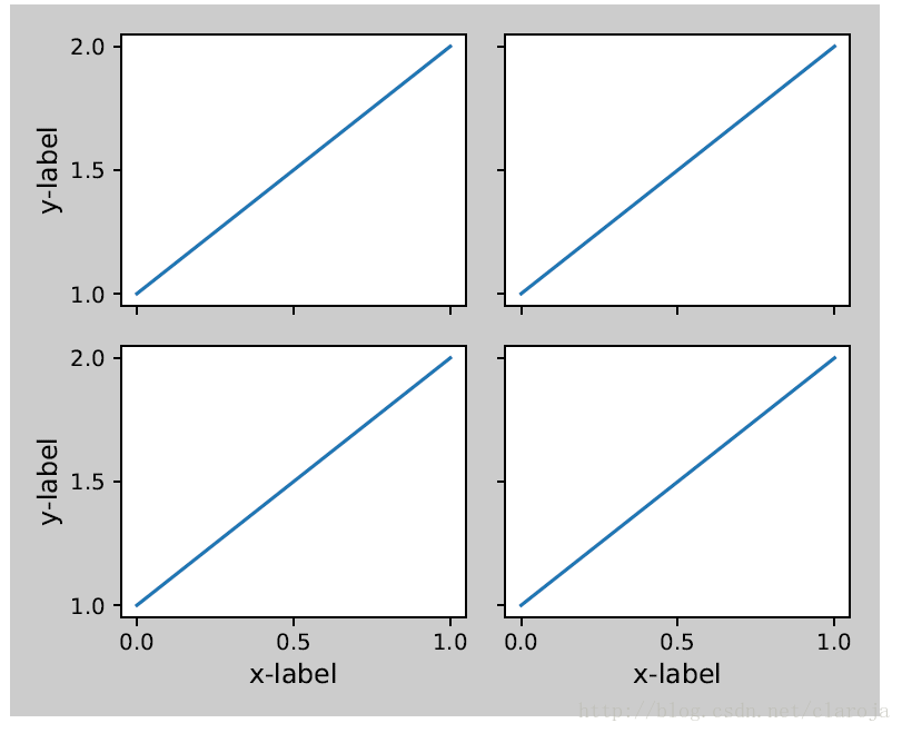

在colorbar中使用tight_layout()

colorbar是Axes的实例，而不是Subplot的实例，所以tight_layout不会起作用，在matplotlib v1.1中，你把colorbar作为一个subplot来使用gridspec。

plt.close('all')
arr = np.arange(100).reshape((10,10))
fig = plt.figure(figsize=(4, 4))
im = plt.imshow(arr, interpolation="none")
plt.colorbar(im, use_gridspec=True)
plt.tight_layout()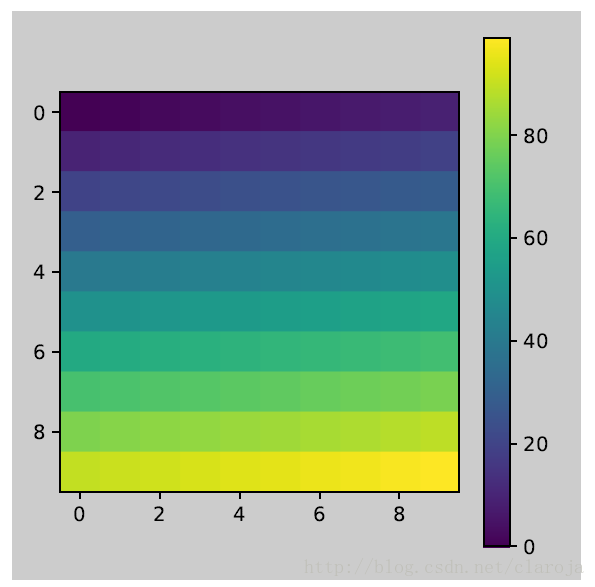

 
另外一个方法是，使用AxesGrid1工具箱为colorbar创建一个轴Axes

plt.close('all')
arr = np.arange(100).reshape((10,10))
fig = plt.figure(figsize=(4, 4))
im = plt.imshow(arr, interpolation="none")
from mpl_toolkits.axes_grid1 import make_axes_locatable
divider = make_axes_locatable(plt.gca())
cax = divider.append_axes("right", "5%", pad="3%")
plt.colorbar(im, cax=cax)
plt.tight_layout()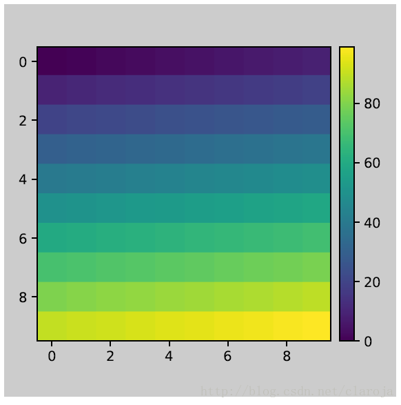

---

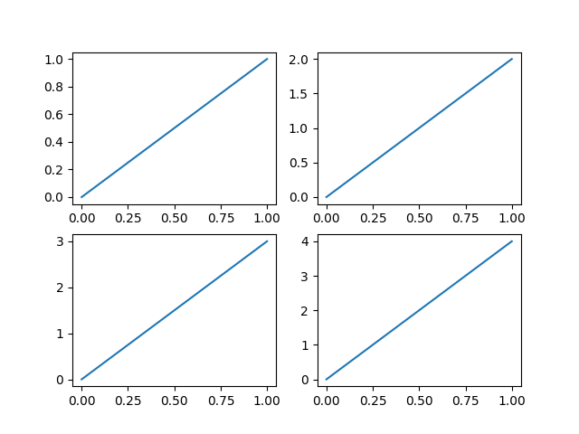
代码：

import matplotlib.pyplot as plt
 
# 多合一显示
# 模式一
plt.figure(1)
plt.subplot(2, 2, 1)
plt.plot([0, 1], [0, 1])
 
plt.subplot(2, 2, 2)
plt.plot([0, 1], [0, 2])
 
plt.subplot(2, 2, 3)
plt.plot([0, 1], [0, 3])
 
plt.subplot(2, 2, 4)
plt.plot([0, 1], [0, 4])
 
# 模式二
plt.figure(2)
plt.subplot(2, 1, 1)
plt.plot([0, 1], [0, 1])
 
plt.subplot(2, 3, 4)
plt.plot([0, 1], [0, 2])
 
plt.subplot(2, 3, 5)
plt.plot([0, 1], [0, 3])
 
plt.subplot(2, 3, 6)
plt.plot([0, 1], [0, 4])
 
plt.show()

运行结果：