笔记:Pytorch官方教程-对抗样本生成
翻译自:https://pytorch.org/tutorials/beginner/fgsm_tutorial.html
尽管深度学习的模型越来越快速、越准确,但深入了解对抗学习之后,你会惊讶的发现,向图像添加微小的难以察觉的扰动可能使模型性能发生显著改变。
这个教程将通过图像分类器来讨论这个问题,具体来说,我们将使用最早的也是最流行的FGSM方法,来愚弄MNIST分类器。
Threat Model
在上下文中,有许多种类的对抗性攻击,每种攻击都有不同的目标和攻击者的知识假设。然而,一般来说,首要目标是对输入数据添加最少的扰动,以导致所需的误分类。
攻击者的知识有几种假设,其中两种是:白盒和黑盒。白盒攻击假定攻击者完全了解和访问模型,包括体系结构、输入、输出和权重。黑盒攻击假定攻击者只能访问模型的输入和输出,而对底层架构或权重一无所知。
还有几种类型的目标,包括错误分类和源/目标错误分类。错误分类的目标意味着对手只希望输出分类是错误的,而不关心新分类是什么。源/目标错误分类意味着对手想要更改最初属于特定源类别的图像,以便将其分类为特定目标类别,可见 https://momodel.cn/workspace/618b8c6d85f93acaac091381?type=app这个例子,非常有趣。
在这种情况下,FGSM攻击是以错误分类为目标的白盒攻击。有了这些背景信息,我们现在可以详细讨论这次攻击
Fast Grandient Sign Attack
这最早且最流行的对抗攻击方式是Fast Grandient Sign Attack(FGSA),它是GoodFellow在 Explaining and Harnessing Adversarial Examples. 中提出的,这种攻击非常强大且很直观。它是通过神经网络本身的学习方式——梯度来进行攻击,它的思路很简单,不是通过反向传播的梯度去调整权重使最小化loss,而是根据梯度来调整输入使得loss最大化.
在开始编写代码之前,让我们先看看著名的FGSM 熊猫例子 和 介绍一些符号公式

根据这张图片,$x$ 是原始的输入图像其分类是"panda",$y$ 是 $x$ 的 $ground truth label$,$\theta$ 指模型的参数,$J(\theta, \mathbf{x}, y)$ 是用来训练网络的loss。攻击将梯度反向传播到输入来计算 loss对 $x$ 的偏导数 $\nabla_{x} J(\theta, \mathbf{x}, y)$,然后,我们将小步($\epsilon$ 或这个例子中的0.7)地调整输入数据,在 $\operatorname{sign}\left(\nabla_{x} J(\theta, \mathbf{x}, y)\right.$ 方向上,从而最大化loss。由此产生的扰动图像 ${x}'$ 将会被目标网络识别成"gibbon"(长臂猿),而人眼看来还是"panda"(熊猫)
希望本教程的动机现在已经很清楚了,让我们开始实现。
Implementation
完整代码可见 https://gist.github.com/growvv/c3188af99b49315423afbd6843fcd05d
FGSM Attack
我们定义一个创建对抗样本的函数,它有三个输入:原始图片 $x$、扰动幅度 $\epsilon$、loss的梯度 ${data_grad}$,创建扰动图像的函数如下:
$$\text { perturbed_image }=\text { image }+\text { epsilon } * \operatorname{sign}(\text { data_grad })=x+\epsilon * \operatorname{sign}\left(\nabla_{x} J(\theta, \mathbf{x}, y)\right)$$
最后,为了保持数据原来的范围,这个扰动图像将截断在 $[0, 1]$
# FGSM attack code
def fgsm_attack(image, epsilon, data_grad):
    # Collect the element-wise sign of the data gradient
    sign_data_grad = data_grad.sign()
    # Create the perturbed image by adjusting each pixel of the input image
    perturbed_image = image + epsilon*sign_data_grad
    # Adding clipping to maintain [0,1] range
    perturbed_image = torch.clamp(perturbed_image, 0, 1)
    # Return the perturbed image
    return perturbed_image
Testing Function
我们会设置不同的 $\epsilon$ 来调用测试函数。测试函数将原来能正确分类的样本加上扰动,达到扰动样本,在将扰动样本进行测试,并且扰动后分类出错的样本保存下来,用于后面的可视化
点击查看代码
def test( model, device, test_loader, epsilon ):

    # Accuracy counter
    correct = 0
    adv_examples = []

    # 一个一个测试, batch_size=1
    for data, target in test_loader:

        data, target = data.to(device), target.to(device)
        # Set requires_grad attribute of tensor. Important for Attack
        data.requires_grad = True

        output = model(data)
        init_pred = output.max(1, keepdim=True)[1] # get the index of the max log-probability

        # 本来就分类错误的话,就不用进行攻击了
        if init_pred.item() != target.item():
            continue

        loss = F.nll_loss(output, target)

        # Zero all existing gradients
        model.zero_grad()

        # Calculate gradients of model in backward pass
        loss.backward()

        # Collect datagrad
        data_grad = data.grad.data

        # Call FGSM Attack
        perturbed_data = fgsm_attack(data, epsilon, data_grad)

        # Re-classify the perturbed image
        output = model(perturbed_data)

        # Check for success
        final_pred = output.max(1, keepdim=True)[1] # get the index of the max log-probability
        if final_pred.item() == target.item():
            correct += 1
            # Special case for saving 0 epsilon examples
            if (epsilon == 0) and (len(adv_examples) < 5):
                adv_ex = perturbed_data.squeeze().detach().cpu().numpy()
                adv_examples.append( (init_pred.item(), final_pred.item(), adv_ex) )
        else:
            # Save some adv examples for visualization later
            if len(adv_examples) < 5:
                adv_ex = perturbed_data.squeeze().detach().cpu().numpy()
                adv_examples.append( (init_pred.item(), final_pred.item(), adv_ex) )

    # Calculate final accuracy for this epsilon
    final_acc = correct/float(len(test_loader))
    print("Epsilon: {}\tTest Accuracy = {} / {} = {}".format(epsilon, correct, len(test_loader), final_acc))

    # Return the accuracy and an adversarial example
    return final_acc, adv_examples
Run Attack
在每个 $\epsilon$ 上进行测试
accuracies = []
examples = []

# Run test for each epsilon
for eps in epsilons:
    acc, ex = test(model, device, test_loader, eps)
    accuracies.append(acc)
    examples.append(ex)
Out:
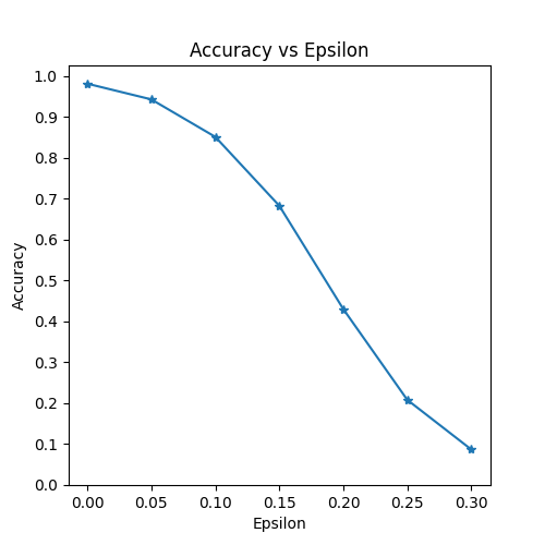
Epsilon: 0      Test Accuracy = 9810 / 10000 = 0.981
Epsilon: 0.05   Test Accuracy = 9426 / 10000 = 0.9426
Epsilon: 0.1    Test Accuracy = 8510 / 10000 = 0.851
Epsilon: 0.15   Test Accuracy = 6826 / 10000 = 0.6826
Epsilon: 0.2    Test Accuracy = 4301 / 10000 = 0.4301
Epsilon: 0.25   Test Accuracy = 2082 / 10000 = 0.2082
Epsilon: 0.3    Test Accuracy = 869 / 10000 = 0.0869
正如预期的一样,$\epsilon$ 越大,准确度会越低,但是注意,并不是线性下降的,尽管 $\epsilon$ 是线性间隔
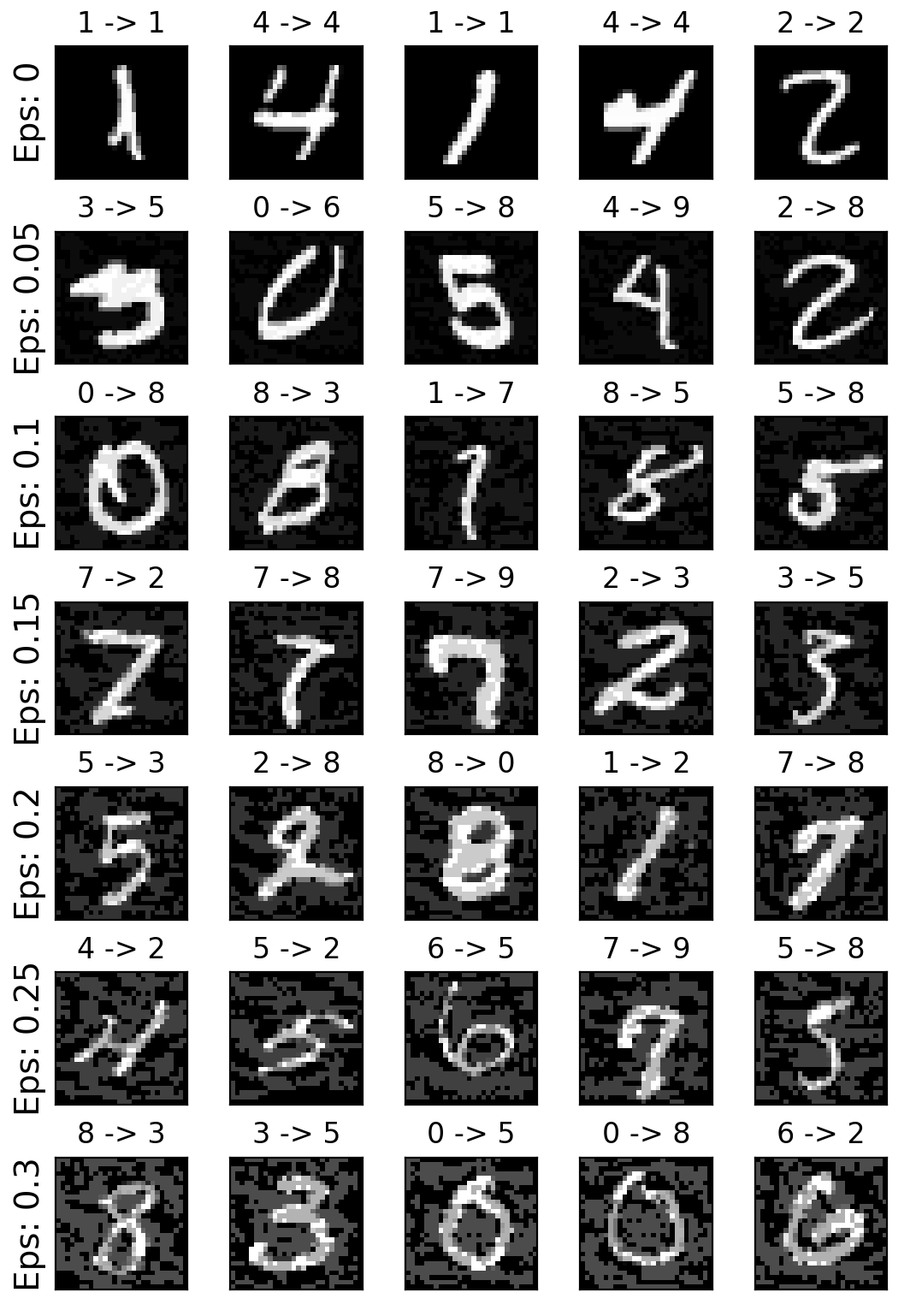
Sample Adversarial Examples
把前面保存的samples可视化,每一类有5张。可以发现,“天下没有免费的午餐”,随着 $\epsilon$ 增大,准确度降低,但扰动变得更容易察觉。在现实中,攻击者必须在准确性和可感知性之间做折中。
Where to go next
这种攻击仅仅代表对抗性攻击研究的开始,因此这随后还有许多想法关于对抗性攻击和防御。事实上,在NIPS 2017上有一个对抗攻击与防御比赛,这篇论文 Adversarial Attacks and Defences Competition 记录了比赛中用到的许多方法。除此之外,这个工作也使得机器学习模型变得更鲁棒,无论是对于自然扰动输入还是恶意输入。
另一个方向是在其他领域使用对抗攻击与防御,比如用到语音和文本。但是学习对抗式机器学习最好的方式是 get your hands dirty,去尝试实现NIPS 2017中其他的attack方式,看它们与FSGM有什么不同,然后尝试防御你自己的攻击.

 浙公网安备 33010602011771号