梯度下降法,牛顿法,高斯-牛顿迭代法,附代码实现 --- --- 转载一片优秀的博客
转载一篇优秀的博客,只为学习目的 !
https://blog.csdn.net/piaoxuezhong/article/details/60135153
---------------------梯度下降法-------------------
梯度的一般解释:
f(x)在x0的梯度:就是f(x)变化最快的方向。梯度下降法是一个最优化算法,通常也称为最速下降法。

假设f(x)是一座山,站在半山腰,往x方向走1米,高度上升0.4米,也就是说x方向上的偏导是 0.4;往y方向走1米,高度上升0.3米,也就是说y方向上的偏导是 0.3;这样梯度方向就是 (0.4 , 0.3),也就是往这个方向走1米,所上升的高度最高。梯度不仅仅是f(x)在某一点变化最快的方向,而且是上升最快的方向;如果想下山,下降最快的方向就是逆着梯度的方向,这就是梯度下降法,又叫最速下降法。
梯度下降法用途:
最速下降法是求解无约束优化问题最简单和最古老的方法之一,虽然现在已经不具有实用性,但是许多有效算法都是以它为基础进行改进和修正而得到的。最速下降法是用负梯度方向为搜索方向的,最速下降法越接近目标值,步长越小,前进越慢。
迭代公式:
其中,λ为步长,就是每一步走多远,这个参数如果设置的太大,那么很容易就在最优值附加徘徊;相反,如果设置的太小,则会导致收敛速度过慢。所以针对这一现象,也有一些相应的改进算法。例如,改进的随机梯度下降算法,伪代码如下:
/*************************************
初始化回归系数为1
重复下面步骤直到收敛
{
对随机遍历的数据集中的每个样本
随着迭代的逐渐进行,减小alpha的值
计算该样本的梯度
使用alpha x gradient来更新回归系数
}
**************************************/


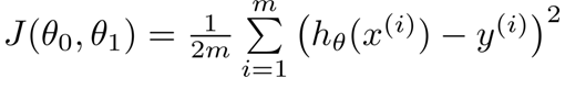
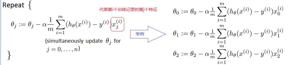
举例说明,定义出多变量线性回归的模型:

梯度下降、随机梯度下降、批量(小批量)梯度下降算法对比:
随机梯度下降:可以看到多了随机两个字,随机也就是说用样本中的一个例子来近似所有的样本,来调整θ,因而随机梯度下降是会带来一定的问题,因为计算得到的并不是准确的一个梯度,容易陷入到局部最优解中
批量梯度下降:其实批量的梯度下降就是一种折中的方法,他用了一些小样本来近似全部的,其本质就是随机指定一个例子替代样本不太准,那我用个30个50个样本那比随机的要准不少了吧,而且批量的话还是非常可以反映样本的一个分布情况的。
------------------------牛顿法------------------------
1、求解方程。
并不是所有的方程都有求根公式,或者求根公式很复杂,导致求解困难。利用牛顿法,可以迭代求解。
原理是利用泰勒公式,在x0处泰勒展开到一阶,即:f(x) = f(x0)+(x-x0)f'(x0)
求解方程:f(x)=0,即:f(x0)+(x-x0)*f'(x0)=0,求解:x = x1=x0-f(x0)/f'(x0),
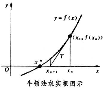
利用泰勒公式的一阶展开,f(x) = f(x0)+(x-x0)f'(x0)处只是近似相等,这里求得的x1并不能让f(x)=0,只能说f(x1)的值比f(x0)更接近f(x)=0,于是乎,迭代求解的想法就很自然了,可以进而推出x(n+1)=x(n)-f(x(n))/f'(x(n)),通过迭代,这个式子必然在f(x*)=0的时候收敛。整个过程如下图:
2、牛顿法用于最优化
在最优化的问题中,线性最优化至少可以使用单纯行法求解,但对于非线性优化问题,牛顿法提供了一种求解的办法。假设任务是优化一个目标函数f,求函数f的极大极小问题,可以转化为求解函数f的导数f'=0的问题,这样求可以把优化问题看成方程求解问题(f'=0)。剩下的问题就和第一部分提到的牛顿法求解很相似了。在极小值估计值附近,把f(x)泰勒展开到2阶形式:
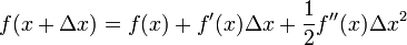
当且仅当 Δx 无线趋近于0,上面的公式成立。令:f'(x+delta(X))=0,得到:

求解:
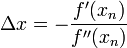
得出迭代公式:

从本质上去看,牛顿法是二阶收敛,梯度下降是一阶收敛,所以牛顿法更快。比如你想找一条最短的路径走到一个盆地的最底部,梯度下降法每次只从你当前所处位置选一个坡度最大的方向走一步,牛顿法在选择方向时,不仅会考虑坡度是否够大,还会考虑你走了一步之后,坡度是否会变得更大。所以,可以说牛顿法比梯度下降法看得更远一点,能更快地走到最底部。(牛顿法目光更加长远,所以少走弯路;相对而言,梯度下降法只考虑了局部的最优,没有全局思想。
从几何上说,牛顿法就是用一个二次曲面去拟合你当前所处位置的局部曲面,而梯度下降法是用一个平面去拟合当前的局部曲面,通常情况下,二次曲面的拟合会比平面更好,所以牛顿法选择的下降路径会更符合真实的最优下降路径。如下图是一个最小化一个目标方程的例子,红色曲线是利用牛顿法迭代求解,绿色曲线是利用梯度下降法求解。

在上面讨论的是2维情况,高维情况的牛顿迭代公式是:

其中H是hessian矩阵,定义为:
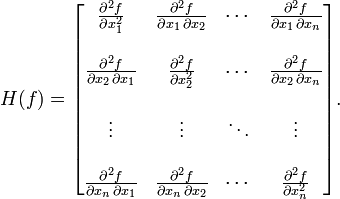
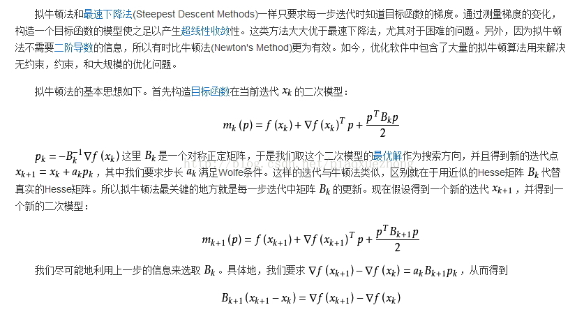
高维情况也可以用牛顿迭代求解,但是Hessian矩阵引入的复杂性,使得牛顿迭代求解的难度增加,解决这个问题的办法是拟牛顿法(Quasi-Newton methond),po下拟牛顿法的百科简述:
----------------高斯-牛顿迭代法----------------
高斯--牛顿迭代法的基本思想是使用泰勒级数展开式去近似地代替非线性回归模型,然后通过多次迭代,多次修正回归系数,使回归系数不断逼近非线性回归模型的最佳回归系数,最后使原模型的残差平方和达到最小。
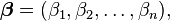
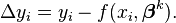
①已知m个点:

②函数原型:
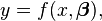
其中:(m>=n),
③目的是找到最优解β,使得残差平方和最小:

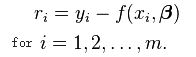
残差:
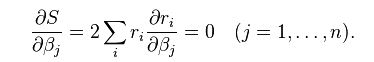
④要求最小值,即S的对β偏导数等于0:
⑤在非线性系统中,
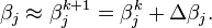
其中k是迭代次数,
⑥每次迭代函数是线性的,在

其中:J是已知的矩阵,为了方便迭代,令
⑦此时残差表示为:

⑧带入公式④有:
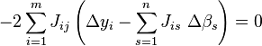
化解得:
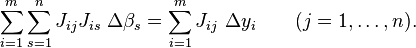
⑨写成矩阵形式:
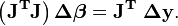
⑩所以最终迭代公式为:

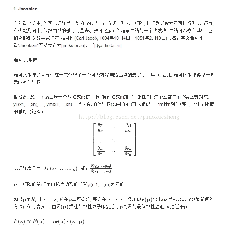
其中,Jf是函数f=(x,β)对β的雅可比矩阵。
关于雅克比矩阵,可以参见一篇写的不错的博文:http://jacoxu.com/jacobian矩阵和hessian矩阵/,这里只po博文里的雅克比矩阵部分:
----------------------代码部分--------------------
1.梯度下降法代码
/*
需要参数为theta:theta0,theta1
目标函数:y=theta0*x0+theta1*x1;
*/
#include <iostream>
using namespace std;

int main()
{
    float matrix[4][2] = { { 1, 1 }, { 2, 1 }, { 2, 2 }, { 3, 4 } };
    float result[4] = {5,6.99,12.02,18};
    float theta[2] = {0,0};
    float loss = 10.0;
    for (int i = 0; i < 10000 && loss>0.0000001; ++i)
    {
        float ErrorSum = 0.0;
        float cost[2] = { 0.0, 0.0 };
        for (int j = 0; j <4; ++j)
        {
            float h = 0.0;
            for (int k = 0; k < 2; ++k)
            {
                h += matrix[j][k] * theta[k];
            }

            ErrorSum = result[j] - h;

            for (int k = 0; k < 2; ++k)
            {
                cost[k] = ErrorSum*matrix[j][k];
            }
        }
        for (int k = 0; k < 2; ++k)
        {
            theta[k] = theta[k] + 0.01*cost[k] / 4;
        }

        cout << "theta[0]=" << theta[0] << "\n" << "theta[1]=" << theta[1] << endl;
        loss = 0.0;
        for (int j = 0; j < 4; ++j)
        {
            float h2 = 0.0;
            for (int k = 0; k < 2; ++k)
            {
                h2 += matrix[j][k] * theta[k];
            }
            loss += (h2 - result[j])*(h2 - result[j]);
        }
        cout << "loss=" << loss << endl;
    }
    return 0;
}
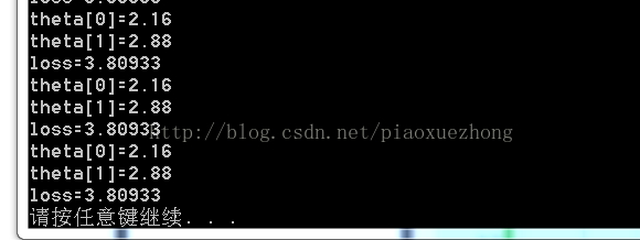
/*
需要参数为theta:theta0,theta1
目标函数:y=theta0*x0+theta1*x1;
*/
#include <iostream>
using namespace std;

int main()
{
    float matrix[4][2] = { { 1, 1 }, { 2, 1 }, { 2, 2 }, { 3, 4 } };
    float result[4] = {5,6.99,12.02,18};
    float theta[2] = {0,0};
    float loss = 10.0;
    for (int i = 0; i<1000 && loss>0.00001; ++i)
    {
        float ErrorSum = 0.0;
        int j = i % 4;

        float h = 0.0;
        for (int k = 0; k<2; ++k)
        {
            h += matrix[j][k] * theta[k];
        }

        ErrorSum = result[j] - h;

        for (int k = 0; k<2; ++k)
        {
            theta[k] = theta[k] + 0.001*(ErrorSum)*matrix[j][k];
        }
        cout << "theta[0]=" << theta[0] << "\n" << "theta[1]=" << theta[1] << endl;

        loss = 0.0;
        for (int j = 0; j<4; ++j)
        {
            float sum = 0.0;
            for (int k = 0; k<2; ++k)
            {

                sum += matrix[j][k] * theta[k];
            }
            loss += (sum - result[j])*(sum - result[j]);
        }
        cout << "loss=" << loss << endl;
    }
    return 0;
}
3.高斯牛顿迭代法代码(见参考目录,暂时只po码)
例子1,根据美国1815年至1885年数据,估计人口模型中的参数A和B。如下表所示,已知年份和人口总量,及人口模型方程,求方程中的参数。
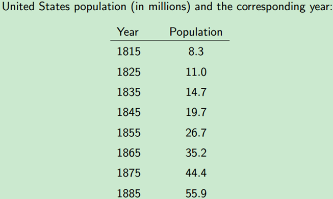
#include <cstdio>

#include <vector>

#include <opencv2/core/core.hpp>


using namespace std;

using namespace cv;


const double DERIV_STEP = 1e-5;

const int MAX_ITER = 100;


void GaussNewton(double(*Func)(const Mat &input, const Mat params),

const Mat &inputs, const Mat &outputs, Mat params);


double Deriv(double(*Func)(const Mat &input, const Mat params),

const Mat &input, const Mat params, int n);


// The user defines their function here

double Func(const Mat &input, const Mat params);


int main()

{

// For this demo we're going to try and fit to the function

// F = A*exp(t*B), There are 2 parameters: A B

int num_params = 2;


// Generate random data using these parameters

int total_data = 8;


Mat inputs(total_data, 1, CV_64F);

Mat outputs(total_data, 1, CV_64F);


//load observation data

for (int i = 0; i < total_data; i++)

{

inputs.at<double>(i, 0) = i + 1; //load year

}

//load America population

outputs.at<double>(0, 0) = 8.3;

outputs.at<double>(1, 0) = 11.0;

outputs.at<double>(2, 0) = 14.7;

outputs.at<double>(3, 0) = 19.7;

outputs.at<double>(4, 0) = 26.7;

outputs.at<double>(5, 0) = 35.2;

outputs.at<double>(6, 0) = 44.4;

outputs.at<double>(7, 0) = 55.9;


// Guess the parameters, it should be close to the true value, else it can fail for very sensitive functions!

Mat params(num_params, 1, CV_64F);


//init guess

params.at<double>(0, 0) = 6;

params.at<double>(1, 0) = 0.3;

GaussNewton(Func, inputs, outputs, params);

printf("Parameters from GaussNewton: %f %f\n", params.at<double>(0, 0), params.at<double>(1, 0));


return 0;

}


double Func(const Mat &input, const Mat params)

{

// Assumes input is a single row matrix

// Assumes params is a column matrix

double A = params.at<double>(0, 0);

double B = params.at<double>(1, 0);

double x = input.at<double>(0, 0);

return A*exp(x*B);

}


//calc the n-th params' partial derivation , the params are our final target

double Deriv(double(*Func)(const Mat &input, const Mat params), const Mat &input, const Mat params, int n)

{

// Assumes input is a single row matrix

// Returns the derivative of the nth parameter

Mat params1 = params.clone();

Mat params2 = params.clone();

// Use central difference to get derivative

params1.at<double>(n, 0) -= DERIV_STEP;

params2.at<double>(n, 0) += DERIV_STEP;

double p1 = Func(input, params1);

double p2 = Func(input, params2);

double d = (p2 - p1) / (2 * DERIV_STEP);

return d;

}


void GaussNewton(double(*Func)(const Mat &input, const Mat params),

const Mat &inputs, const Mat &outputs, Mat params)

{

int m = inputs.rows;

int n = inputs.cols;

int num_params = params.rows;


Mat r(m, 1, CV_64F); // residual matrix

Mat Jf(m, num_params, CV_64F); // Jacobian of Func()

Mat input(1, n, CV_64F); // single row input


double last_mse = 0;


for (int i = 0; i < MAX_ITER; i++)

{

double mse = 0;

for (int j = 0; j < m; j++)

{

for (int k = 0; k < n; k++)

{//copy Independent variable vector, the year

input.at<double>(0, k) = inputs.at<double>(j, k);

}

r.at<double>(j, 0) = outputs.at<double>(j, 0) - Func(input, params);//diff between estimate and observation population

mse += r.at<double>(j, 0)*r.at<double>(j, 0);

for (int k = 0; k < num_params; k++)

{

Jf.at<double>(j, k) = Deriv(Func, input, params, k);

}

}


mse /= m;

// The difference in mse is very small, so quit

if (fabs(mse - last_mse) < 1e-8)

{

break;

}


Mat delta = ((Jf.t()*Jf)).inv() * Jf.t()*r;

params += delta;

//printf("%d: mse=%f\n", i, mse);

printf("%d %f\n", i, mse);

last_mse = mse;

}

}
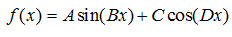
例子2:要拟合如下模型,
由于缺乏观测量,就自导自演,假设4个参数已知A=5,B=1,C=10,D=2,构造100个随机数作为x的观测值,计算相应的函数观测值。然后,利用这些观测值,反推4个参数。
#include <cstdio>

#include <vector>

#include <opencv2/core/core.hpp>


using namespace std;

using namespace cv;


const double DERIV_STEP = 1e-5;

const int MAX_ITER = 100;


void GaussNewton(double(*Func)(const Mat &input, const Mat params),

const Mat &inputs, const Mat &outputs, Mat params);


double Deriv(double(*Func)(const Mat &input, const Mat params),

const Mat &input, const Mat params, int n);


double Func(const Mat &input, const Mat params);


int main()

{

// For this demo we're going to try and fit to the function

// F = A*sin(Bx) + C*cos(Dx),There are 4 parameters: A, B, C, D

int num_params = 4;

// Generate random data using these parameters

int total_data = 100;


double A = 5;

double B = 1;

double C = 10;

double D = 2;


Mat inputs(total_data, 1, CV_64F);

Mat outputs(total_data, 1, CV_64F);


for (int i = 0; i < total_data; i++) {

double x = -10.0 + 20.0* rand() / (1.0 + RAND_MAX); // random between [-10 and 10]

double y = A*sin(B*x) + C*cos(D*x);

// Add some noise

// y += -1.0 + 2.0*rand() / (1.0 + RAND_MAX);

inputs.at<double>(i, 0) = x;

outputs.at<double>(i, 0) = y;

}

// Guess the parameters, it should be close to the true value, else it can fail for very sensitive functions!

Mat params(num_params, 1, CV_64F);

params.at<double>(0, 0) = 1;

params.at<double>(1, 0) = 1;

params.at<double>(2, 0) = 8; // changing to 1 will cause it not to find the solution, too far away

params.at<double>(3, 0) = 1;

GaussNewton(Func, inputs, outputs, params);

printf("True parameters: %f %f %f %f\n", A, B, C, D);

printf("Parameters from GaussNewton: %f %f %f %f\n", params.at<double>(0, 0), params.at<double>(1, 0),

params.at<double>(2, 0), params.at<double>(3, 0));


return 0;

}


double Func(const Mat &input, const Mat params)

{

// Assumes input is a single row matrix

// Assumes params is a column matrix

double A = params.at<double>(0, 0);

double B = params.at<double>(1, 0);

double C = params.at<double>(2, 0);

double D = params.at<double>(3, 0);

double x = input.at<double>(0, 0);

return A*sin(B*x) + C*cos(D*x);

}


double Deriv(double(*Func)(const Mat &input, const Mat params), const Mat &input, const Mat params, int n)

{

// Assumes input is a single row matrix

// Returns the derivative of the nth parameter

Mat params1 = params.clone();

Mat params2 = params.clone();

// Use central difference to get derivative

params1.at<double>(n, 0) -= DERIV_STEP;

params2.at<double>(n, 0) += DERIV_STEP;

double p1 = Func(input, params1);

double p2 = Func(input, params2);

double d = (p2 - p1) / (2 * DERIV_STEP);

return d;

}


void GaussNewton(double(*Func)(const Mat &input, const Mat params),

const Mat &inputs, const Mat &outputs, Mat params)

{

int m = inputs.rows;

int n = inputs.cols;

int num_params = params.rows;

Mat r(m, 1, CV_64F); // residual matrix

Mat Jf(m, num_params, CV_64F); // Jacobian of Func()

Mat input(1, n, CV_64F); // single row input


double last_mse = 0;


for (int i = 0; i < MAX_ITER; i++)

{

double mse = 0;

for (int j = 0; j < m; j++)

{

for (int k = 0; k < n; k++)

{

input.at<double>(0, k) = inputs.at<double>(j, k);

}

r.at<double>(j, 0) = outputs.at<double>(j, 0) - Func(input, params);

mse += r.at<double>(j, 0)*r.at<double>(j, 0);

for (int k = 0; k < num_params; k++)

{

Jf.at<double>(j, k) = Deriv(Func, input, params, k);

}

}

mse /= m;

// The difference in mse is very small, so quit

if (fabs(mse - last_mse) < 1e-8)

{

break;

}

Mat delta = ((Jf.t()*Jf)).inv() * Jf.t()*r;

params += delta;

printf("%f\n", mse);

last_mse = mse;

}

}
参考:
http://blog.csdn.net/xiazdong/article/details/7950084
https://en.wikipedia.org/wiki/Gauss%E2%80%93Newton_algorithm
http://blog.csdn.NET/dsbatigol/article/details/12448627
http://blog.csdn.Net/hbtj_1216/article/details/51605155
http://blog.csdn.net/zouxy09/article/details/20319673
http://blog.chinaunix.net/uid-20648405-id-1907335.html
http://www.2cto.com/kf/201302/189671.html
http://www.cnblogs.com/sylvanas2012/p/logisticregression.html
http://blog.csdn.net/u012328159/article/details/51613262
2.牛顿法代码参考
https://wenku.baidu.com/view/949c00fda1c7aa00b42acb13.html
http://www.2cto.com/kf/201302/189671.html
3.高斯牛顿迭代法代码参考
http://blog.csdn.net/tclxspy/article/details/51281811
http://blog.csdn.net/jinshengtao/article/details/51615162
每一个不曾起舞的日子,都是对生命的辜负。
But it is the same with man as with the tree. The more he seeks to rise into the height and light, the more vigorously do his roots struggle earthward, downward, into the dark, the deep - into evil.
其实人跟树是一样的,越是向往高处的阳光,它的根就越要伸向黑暗的地底。----尼采

 浙公网安备 33010602011771号