算法模型补充

概要

• 模型的假设检验（F与T）

• 岭回归与Lasso回归

• Logistic回归模型

• 决策树与随机森林

• K近邻模型

 

---

详情

• 模型的假设检验（F与T）

F检验

F检验：提出原假设（不合理）和备择假设（合理），之后计算实际值与理论值，通过比较两者判断模型是否合理。

计算实际值

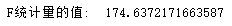
# 需要导入相关模块
import numpy as np
import pandas as pd
from sklearn import model_selection
import statsmodels.api as sm
# 读取数据
pt = pd.read_excel(r'Predict to Profit.xlsx')
# 拆分训练集与测试集
train,test = model_selection.train_test_split(pt,test_size=0.2,random_state=1234)
# 建立模型
pModel = sm.formula.ols('Profit~RD_Spend+Administration+Marketing_Spend+C(State)',data=train).fit()
# 计算建模中因变量的均值
yMean = train.Profit.mean() # 115525.98769230771
# 统计变量个数与观测个数
p = pModel.df_model  # 5
n = train.shape[0]   # 39
# 计算回归离差平方和 52067443965.96364
RSS = np.sum((pModel.fittedvalues-yMean)**2)
# 计算误差平方和 1967765724.576366
ESS = np.sum(pModel.resid**2)
# 计算F实际值
F = (RSS/p)/(ESS/(n-p-1))
print('F统计量的值: ', F)

计算理论值

# 导⼊模块
from scipy.stats import f
# 计算F理论值
FT = f.ppf(q=0.95,dfn = p,dfd = n-p-1)
print('F理论值为: ', FT)

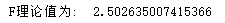
结论：计算出来的F统计量值174.64远远⼤于F分布的理论值2.50 所以应当拒绝原假设（先假设模型不合理）,即多元线性回归模型是显著的，偏回归系数不全为0。

T检验

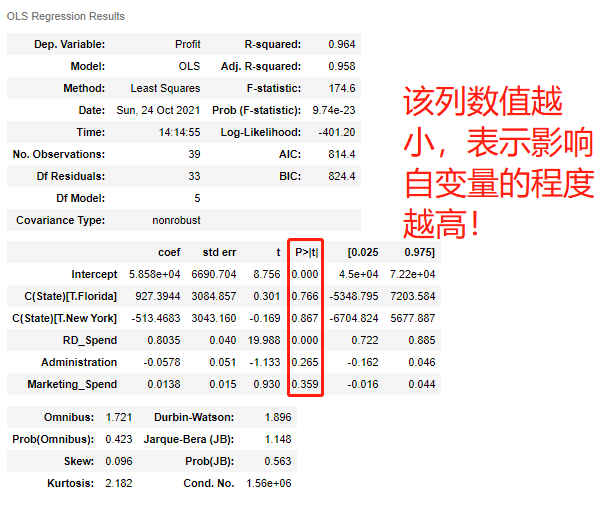
"""T检验更加侧重于检验模型的各个参数是否合理"""
model.summary()  # 结果中P>|t|的绝对值越小对自变量的影响越大

线性回归模型的短板

虽然有上述方法来检验模型以及参数的合理性，线性回归模型依旧存在不适用的场合。

　　1、自变量个数大于样本量。

　　2、自变量直接存在多重共线性（值高度相关）。

为了解决上述问题，需要使用岭回归模型与Lasso回归模型。

---

• 岭回归与Lasso回归

岭回归模型

在线性回归模型的基础之上添加一个l2惩罚项（也称平方项、正则项）。

线性回归模型:J(β)=∑(y−Xβ)^2

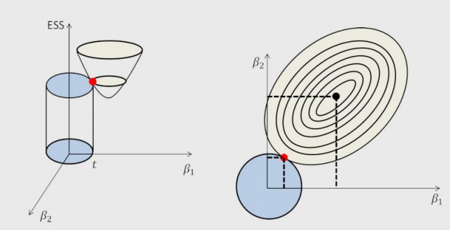
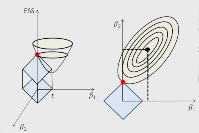
岭回归模型:J(β)=∑(y−Xβ)^2+∑λβ^2

该模型最终转变成求解圆柱体与椭圆抛物线的交点问题，始终保留建模时的所有变量，无法降低模型的复杂度。

岭回归交叉验证的参数

 

RidgeCV(alphas=(0.1, 1.0, 10.0), fit_intercept=True, normalize=False,
scoring=None, cv=None)
# 参数
alphas：⽤于指定多个lambda值的元组或数组对象，默认该参数包含0.1、1和10三种值。
fit_intercept：bool类型参数，是否需要拟合截距项，默认为True。
normalize：bool类型参数，建模时是否需要对数据集做标准化处理，默认为False。
scoring：指定⽤于评估模型的度量⽅法。
cv：指定交叉验证的重数。

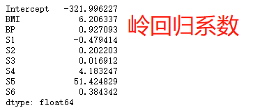
岭回归模型案例

'''求最准确的Lamda值'''
# 导入模块
from sklearn.linear_model import Ridge,RidgeCV
# 读取糖尿病数据集
diabetes = pd.read_excel(r'diabetes.xlsx')
# 构造自变量（剔除患者性别、年龄和因变量）
predictors = diabetes.columns[2:-1]
# 将数据集拆分为训练集和测试集
X_train, X_test, y_train, y_test = model_selection.train_test_split(diabetes[predictors], diabetes['Y'],test_size = 0.2, random_state = 1234)
# 构造不同的Lamda值
Lambdas=np.logspace(-5,2,200)
# 设置交叉验证的参数，对于每一个Lambda值，都执行10重交叉验证
ridge_cv = RidgeCV(alphas = Lambdas, normalize=True, scoring='neg_mean_squared_error', cv = 10)
# 模型拟合
ridge_cv.fit(X_train, y_train)
# 返回最佳的lambda值
ridge_best_Lambda = ridge_cv.alpha_
ridge_best_Lambda # 0.014649713983072863
​
'''基于最准确的Lamda值建模'''
# 导入第三方包中的函数
from sklearn.metrics import mean_squared_error
# 基于最佳的Lambda值建模
ridge = Ridge(alpha = ridge_best_Lambda, normalize=True)
ridge.fit(X_train, y_train)
# 返回岭回归系数
pd.Series(index = ['Intercept'] + X_train.columns.tolist(),data = [ridge.intercept_] + ridge.coef_.tolist())
# 预测
ridge_predict = ridge.predict(X_test)
# 预测效果验证:均方根误差
RMSE = np.sqrt(mean_squared_error(y_test,ridge_predict))
RMSE # 53.119117887535204

Lasso回归模型

在线性回归模型的基础之上添加一个l1惩罚项（也称正则项）。

Lasso回归模型:J(β)=∑(y−Xβ)^2+∑λ|β| 该模型最终转变成求解正方体与椭圆抛物线的交点问题，相较于岭回归降低了模型的复杂度。

Lasso回归交叉验证的参数

LassoCV(alphas=None, fit_intercept=True, 
normalize=False,max_iter=1000, tol=0.0001)
# 参数
alphas：指定具体的Lambda值列表⽤于模型的运算
fit_intercept：bool类型参数，是否需要拟合截距项，默认为True
normalize：bool类型参数，建模时是否需要对数据集做标准化处理，默认为False
max_iter：指定模型最⼤的迭代次数，默认为1000次

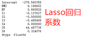
Lasso回归模型案例

'''求最准确的Lamda值'''
# 导入第三方模块中的函数
from sklearn.linear_model import Lasso,LassoCV
# LASSO回归模型的交叉验证
lasso_cv = LassoCV(alphas = Lambdas, normalize=True, cv = 10, max_iter=10000)
lasso_cv.fit(X_train, y_train)
# 输出最佳的lambda值
lasso_best_alpha = lasso_cv.alpha_
lasso_best_alpha # 0.06294988990221888
​
'''基于最准确的Lamda值建模'''
# 基于最佳的lambda值建模
lasso = Lasso(alpha = lasso_best_alpha, normalize=True, max_iter=10000)
lasso.fit(X_train, y_train)
# 返回LASSO回归的系数
xs=pd.Series(index = ['Intercept'] + X_train.columns.tolist(),data = [lasso.intercept_] + lasso.coef_.tolist())
xs
# 预测
lasso_predict = lasso.predict(X_test)
# 预测效果验证
RMSE = np.sqrt(mean_squared_error(y_test,lasso_predict))
RMSE # 53.06143725822573

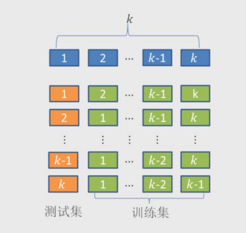
交叉验证的思想

1.将数据集拆分成k个样本量相当的数据组，组件无重叠样本。
2.从k组数据中挑选k-1组用于构建模型，剩下一组用于测试。
3.以此类推，会获得k种训练集和测试集，每一个数据组都将参与构建以及测试。
4.从中选择准确度最高的模型。

---

• Logistic回归模型

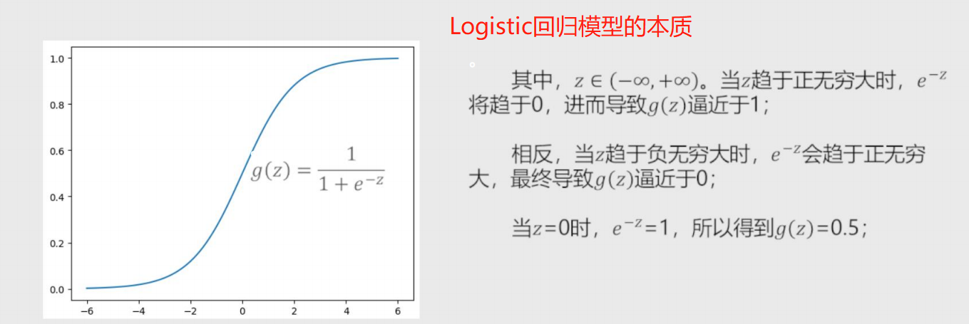
将线性回归模型的公式做Logit变换即为Logistic回归模型

原本的线性回归模型：y = β + β1x1 + β2x2 + ... + βpxp

Logit编号：g(y) = 1/(1+e^(-y)) = hβ(x)

hβ(x)称为Logistic回归模型，将预测问题变成了0到1之间的概率问题。

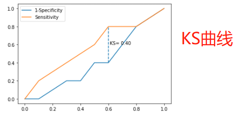
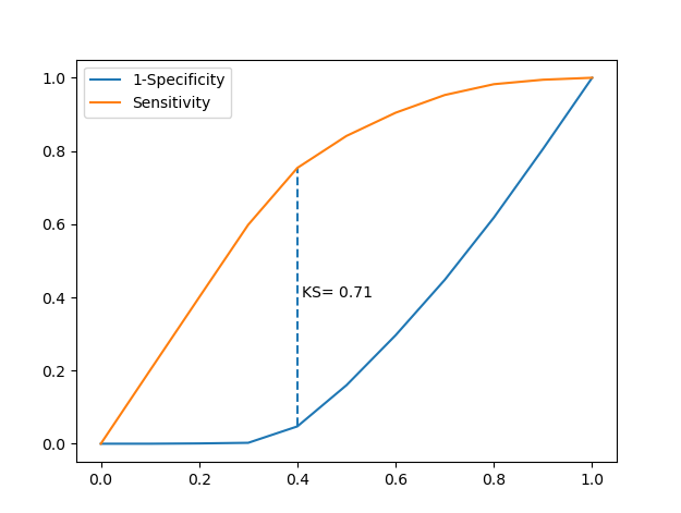
自定义绘制ks曲线的函数

# 导入第三方模块
import pandas as pd
import numpy as np
import matplotlib.pyplot as plt
from sklearn import model_selection
from sklearn import linear_model
​
# 自定义绘制ks曲线的函数
def plot_ks(y_test, y_score, positive_flag):
    # 对y_test重新设置索引
    y_test.index = np.arange(len(y_test))
    # 构建目标数据集
    target_data = pd.DataFrame({'y_test':y_test, 'y_score':y_score})
    # 按y_score降序排列
    target_data.sort_values(by = 'y_score', ascending = False, inplace = True)
    # 自定义分位点
    cuts = np.arange(0.1,1,0.1)
    # 计算各分位点对应的Score值
    index = len(target_data.y_score)*cuts
    scores = np.array(target_data.y_score)[index.astype('int')]
    # 根据不同的Score值，计算Sensitivity和Specificity
    Sensitivity = []
    Specificity = []
    for score in scores:
        # 正例覆盖样本数量与实际正例样本量
        positive_recall = target_data.loc[(target_data.y_test == positive_flag) & (target_data.y_score>score),:].shape[0]
        positive = sum(target_data.y_test == positive_flag)
        # 负例覆盖样本数量与实际负例样本量
        negative_recall = target_data.loc[(target_data.y_test != positive_flag) & (target_data.y_score<=score),:].shape[0]
        negative = sum(target_data.y_test != positive_flag)
        Sensitivity.append(positive_recall/positive)
        Specificity.append(negative_recall/negative)
    # 构建绘图数据
    plot_data = pd.DataFrame({'cuts':cuts,'y1':1-np.array(Specificity),'y2':np.array(Sensitivity), 
                              'ks':np.array(Sensitivity)-(1-np.array(Specificity))})
    # 寻找Sensitivity和1-Specificity之差的最大值索引
    max_ks_index = np.argmax(plot_data.ks)
    plt.plot([0]+cuts.tolist()+[1], [0]+plot_data.y1.tolist()+[1], label = '1-Specificity')
    plt.plot([0]+cuts.tolist()+[1], [0]+plot_data.y2.tolist()+[1], label = 'Sensitivity')
    # 添加参考线
    plt.vlines(plot_data.cuts[max_ks_index], ymin = plot_data.y1[max_ks_index], 
               ymax = plot_data.y2[max_ks_index], linestyles = '--')
    # 添加文本信息
    plt.text(x = plot_data.cuts[max_ks_index]+0.01,
             y = plot_data.y1[max_ks_index]+plot_data.ks[max_ks_index]/2,
             s = 'KS= %.2f' %plot_data.ks[max_ks_index])
    # 显示图例
    plt.legend()
    # 显示图形
    plt.show()

构建模型

案例1-绘制ks曲线

# 导入虚拟数据
virtual_data = pd.read_excel(r'virtual_data.xlsx')
# 应用自定义函数绘制k-s曲线
plot_ks(y_test = virtual_data.Class, y_score = virtual_data.Score,positive_flag = 'P')

案例2-求解模型参数

# 读取数据
sports = pd.read_csv(r'Run or Walk.csv')
# 提取出所有自变量名称
predictors = sports.columns[4:]
# 构建自变量矩阵
X = sports.ix[:,predictors]
# 提取y变量值
y = sports.activity
# 将数据集拆分为训练集和测试集
X_train, X_test, y_train, y_test = model_selection.train_test_split(X, y, test_size = 0.25, random_state = 1234)
​
# 利用训练集建模
sklearn_logistic = linear_model.LogisticRegression()
sklearn_logistic.fit(X_train, y_train)
# 返回模型的各个参数
print(sklearn_logistic.intercept_, sklearn_logistic.coef_)

Logistic回归模型参数

LogisticRegression(tol=0.0001, fit_intercept=True,class_weight=None, max_iter=100)
# 参数
tol：⽤于指定模型跌倒收敛的阈值
fit_intercept：bool类型参数，是否拟合模型的截距项，默认为True
class_weight：⽤于指定因变量类别的权重，如果为字典，则通过字典的形式{class_label:weight}传递每个类别的权重；如果为字符串'balanced'，则每个分类的权重与实际样本中的⽐例成反⽐，当各分类存在严重不平衡时，设置为'balanced'会⽐较好；如果为None，则表示每个分类的权重相等
max_iter：指定模型求解过程中的最⼤迭代次数， 默认为100

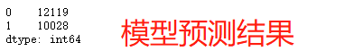
模型预测结果统计

# 模型预测
sklearn_predict = sklearn_logistic.predict(X_test)
# 预测结果统计
pd.Series(sklearn_predict).value_counts()

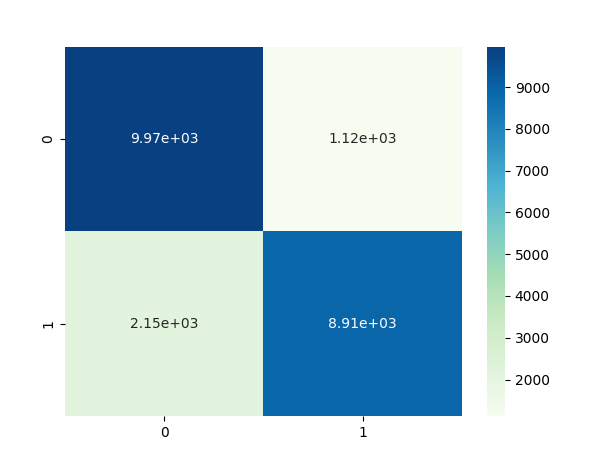
混淆矩阵

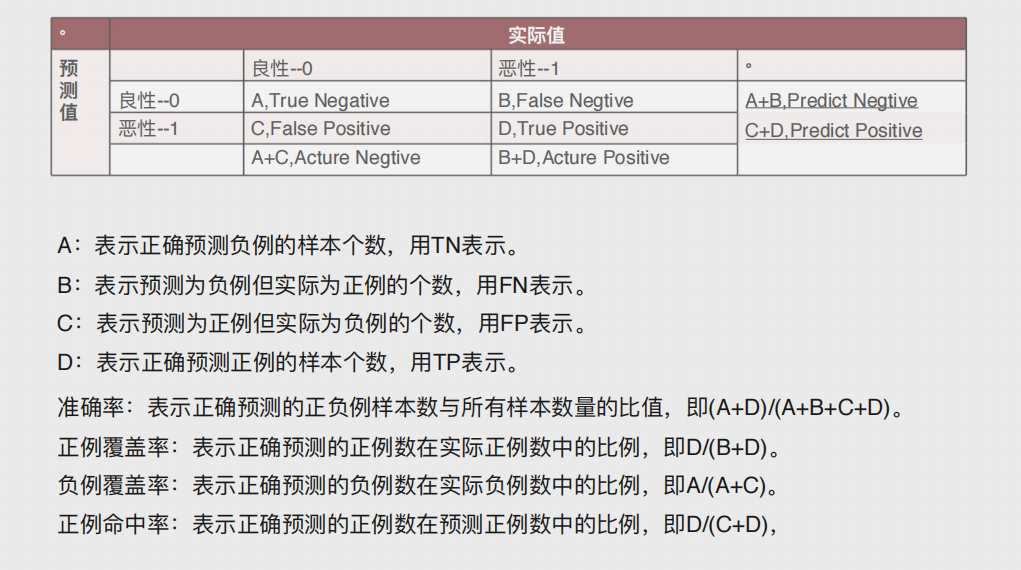
# 导入第三方模块
from sklearn import metrics
# 混淆矩阵
cm = metrics.confusion_matrix(y_test, sklearn_predict, labels = [0,1])

模型准确率以及正反例覆盖率

Accuracy = metrics.scorer.accuracy_score(y_test, sklearn_predict)
Sensitivity = metrics.scorer.recall_score(y_test, sklearn_predict)
Specificity = metrics.scorer.recall_score(y_test, sklearn_predict, pos_label=0)
print('模型准确率为%.2f%%:' %(Accuracy*100))
print('正例覆盖率为%.2f%%' %(Sensitivity*100))
print('负例覆盖率为%.2f%%' %(Specificity*100))

混淆矩阵的可视化—热力图

# 混淆矩阵的可视化
# 导入第三方模块
import seaborn as sns
import matplotlib.pyplot as plt
%matplotlib
# 绘制热力图
sns.heatmap(cm, annot = True, fmt = '.2e',cmap = 'GnBu')
# 图形显示
plt.show()

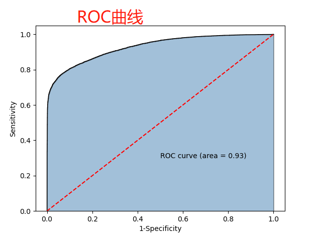
ROC曲线—面积图

计算折线下的⾯积，即阴影部分，这个⾯积称为AUC。

在做模型评估时，希望AUC的值越⼤越好，通常情况下，

当AUC在0.8以上时，说明模型基本准确。

# y得分为模型预测正例的概率
y_score = sklearn_logistic.predict_proba(X_test)[:,1]
# 计算不同阈值下，fpr和tpr的组合值，其中fpr表示1-Specificity，tpr表示Sensitivity
fpr,tpr,threshold = metrics.roc_curve(y_test, y_score)
# 计算AUC的值
roc_auc = metrics.auc(fpr,tpr)
​
# 绘制面积图
plt.stackplot(fpr, tpr, color='steelblue', alpha = 0.5, edgecolor = 'black')
# 添加边际线
plt.plot(fpr, tpr, color='black', lw = 1)
# 添加对角线
plt.plot([0,1],[0,1], color = 'red', linestyle = '--')
# 添加文本信息
plt.text(0.5,0.3,'ROC curve (area = %0.2f)' % roc_auc)
# 添加x轴与y轴标签
plt.xlabel('1-Specificity')
plt.ylabel('Sensitivity')
# 显示图形
plt.show()

# 调用自定义函数，绘制K-S曲线
plot_ks(y_test = y_test, y_score = y_score, positive_flag = 1)

Logistic回归模型的求解流程

# -----------------------第一步 建模 ----------------------- #
# 导入第三方模块
import statsmodels.api as sm
# 将数据集拆分为训练集和测试集
X_train, X_test, y_train, y_test = model_selection.train_test_split(X, y, test_size = 0.25, random_state = 1234)
# 为训练集和测试集的X矩阵添加常数列1
X_train2 = sm.add_constant(X_train)
X_test2 = sm.add_constant(X_test)
# 拟合Logistic模型
sm_logistic = sm.Logit(y_train, X_train2).fit()
# 返回模型的参数
sm_logistic.params
​
# -----------------------第二步 预测构建混淆矩阵 ----------------------- #
# 模型在测试集上的预测
sm_y_probability = sm_logistic.predict(X_test2)
# 根据概率值，将观测进行分类，以0.5作为阈值
sm_pred_y = np.where(sm_y_probability >= 0.5, 1, 0)
# 混淆矩阵
cm = metrics.confusion_matrix(y_test, sm_pred_y, labels = [0,1])
cm
​
# -----------------------第三步 绘制ROC曲线 ----------------------- #
# 计算真正率和假正率 
fpr,tpr,threshold = metrics.roc_curve(y_test, sm_y_probability)
# 计算auc的值  
roc_auc = metrics.auc(fpr,tpr)
# 绘制面积图
plt.stackplot(fpr, tpr, color='steelblue', alpha = 0.5, edgecolor = 'black')
# 添加边际线
plt.plot(fpr, tpr, color='black', lw = 1)
# 添加对角线
plt.plot([0,1],[0,1], color = 'red', linestyle = '--')
# 添加文本信息
plt.text(0.5,0.3,'ROC curve (area = %0.2f)' % roc_auc)
# 添加x轴与y轴标签
plt.xlabel('1-Specificity')
plt.ylabel('Sensitivity')
# 显示图形
plt.show()
​
# -----------------------第四步 绘制K-S曲线 ----------------------- #
# 调用自定义函数，绘制K-S曲线
sm_y_probability.index = np.arange(len(sm_y_probability))
plot_ks(y_test = y_test, y_score = sm_y_probability, positive_flag = 1)
​
""" 模型评估方法 """
1.ROC曲线：通过计算AUC阴影部分的面积来判断模型是否合理(通常大于0.8表示OK)
2.KS曲线：通过计算两条折现之间最大距离来衡量模型是否合理(通常大于0.4表示OK)

---

• 决策树与随机森林

决策树与随机森林：顾名思义，通常用于解决分类（决策）问题，即买不买，带不带，走不走等；也可以用来解决预测问题，即具体数值。

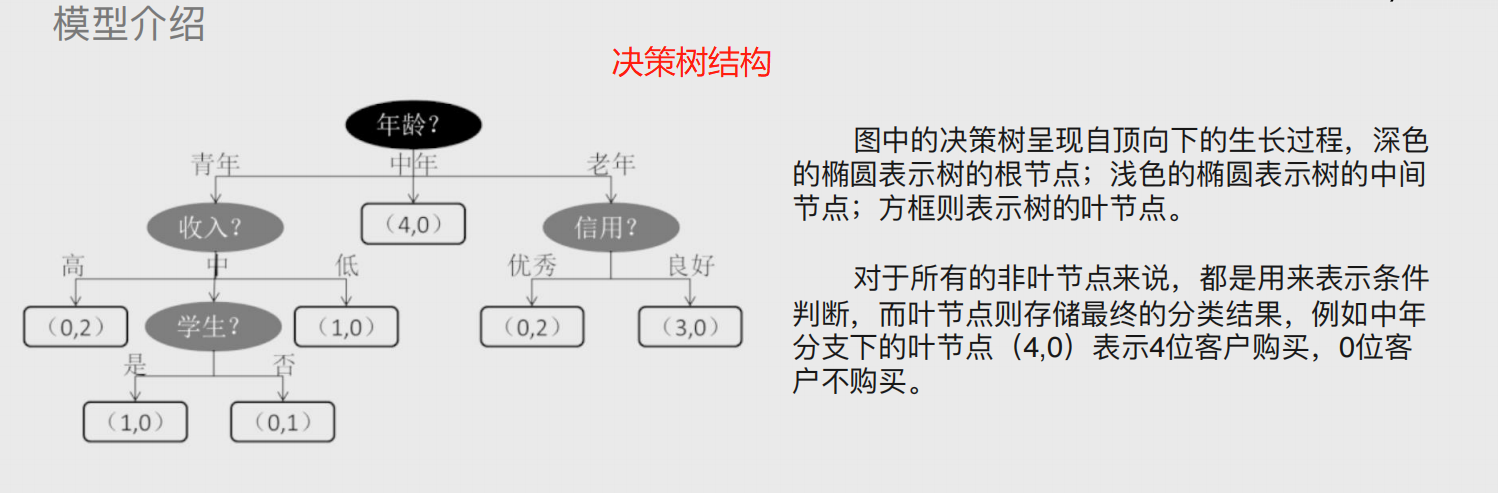
树的概念

这里的树其实是计算机底层的一种数据结构，与现实不同，可理解为自上而下生长
# 决策树
算法模型的概念，由三部分组成
根节点:树的起点
枝节点:即中间节点，和根节点一样也是条件判断
叶子节点:分支的终点

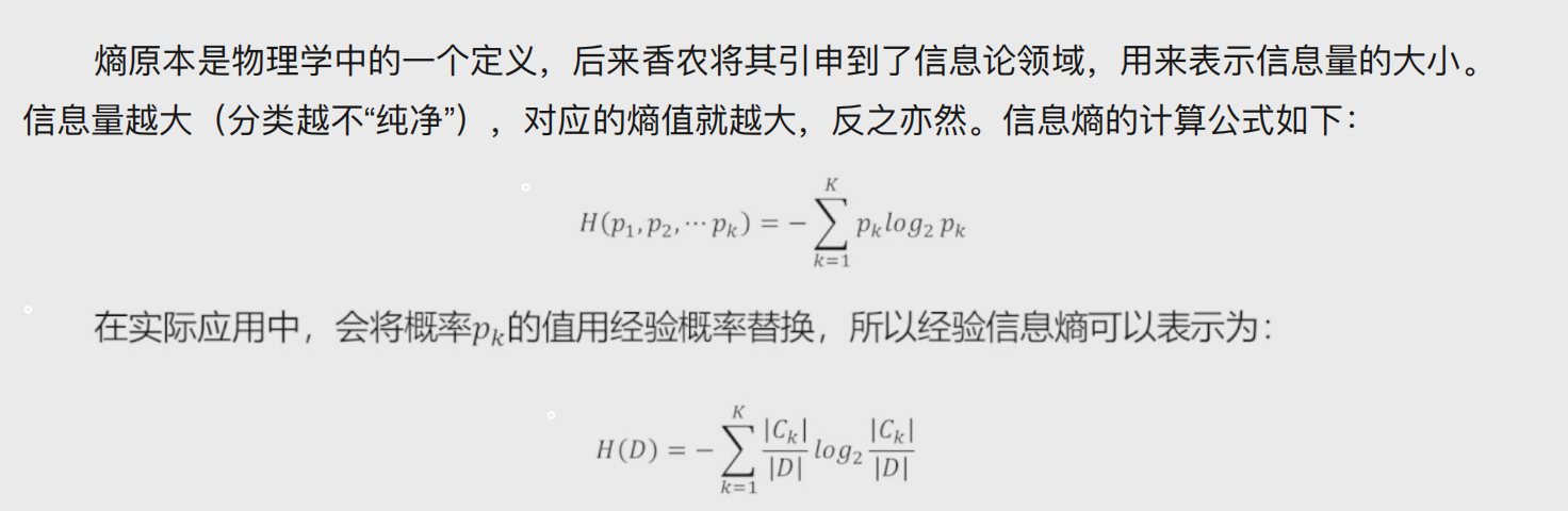
信息熵

熵原本是物理学概念，表示混乱程度；后被引用至信息领域，表示信息量的大小。

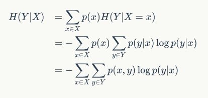
条件熵

条件熵为信息熵的引申，指添加条件后对信息熵进行分类。

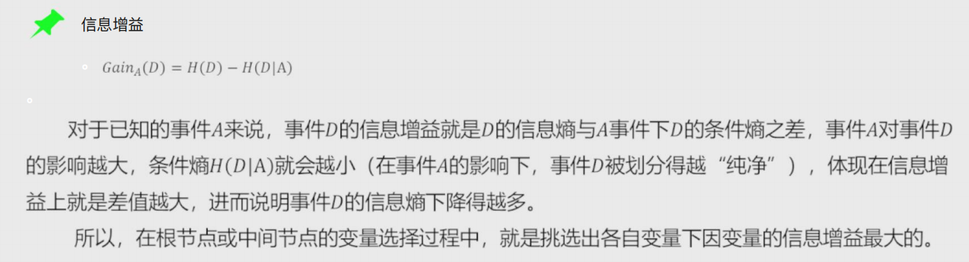
信息增益

用某个条件对原变量分类后，降低了原变量的不确定性。结论，不确定性减少程度就是信息的增益。

构建决策树时，根节点与枝节点存储的条件按照信息增益从大到小排列，即影响越大的条件在构建决策树的时候越靠近根节点！！！

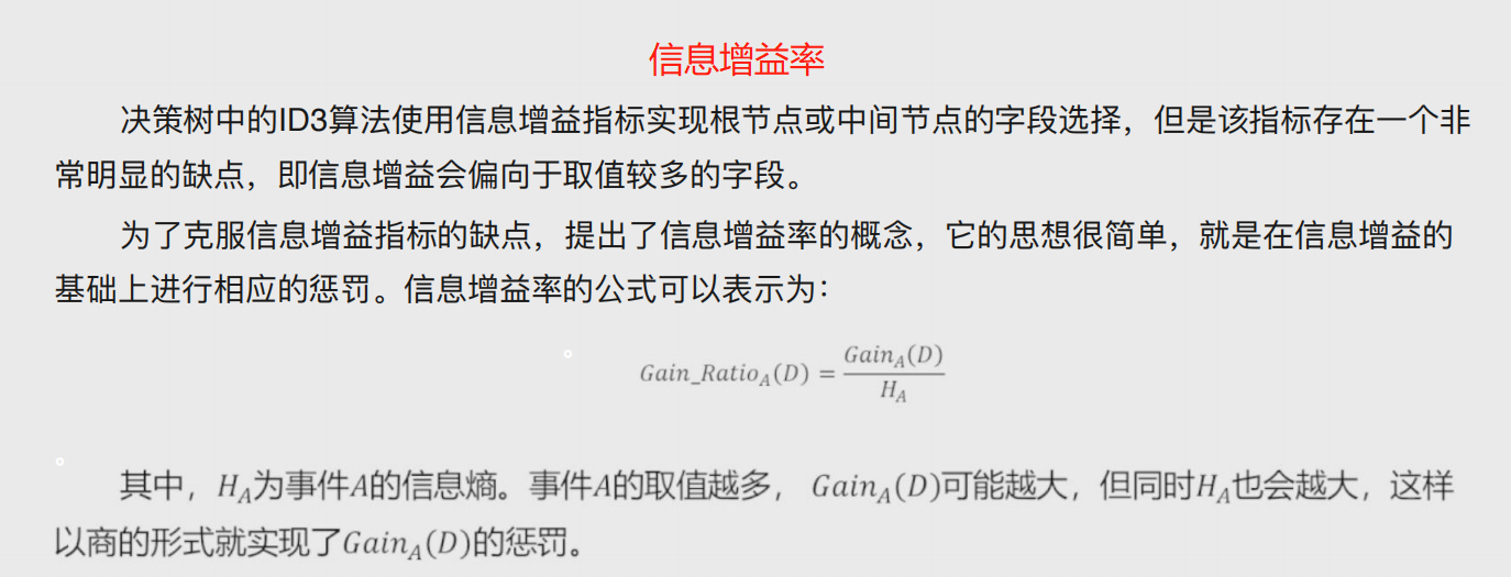
信息增益率

信息增益会偏向于取值较多的字段，为了避免，提出了信息增益率的概念，就是在计算信息增益时添加的惩罚项。

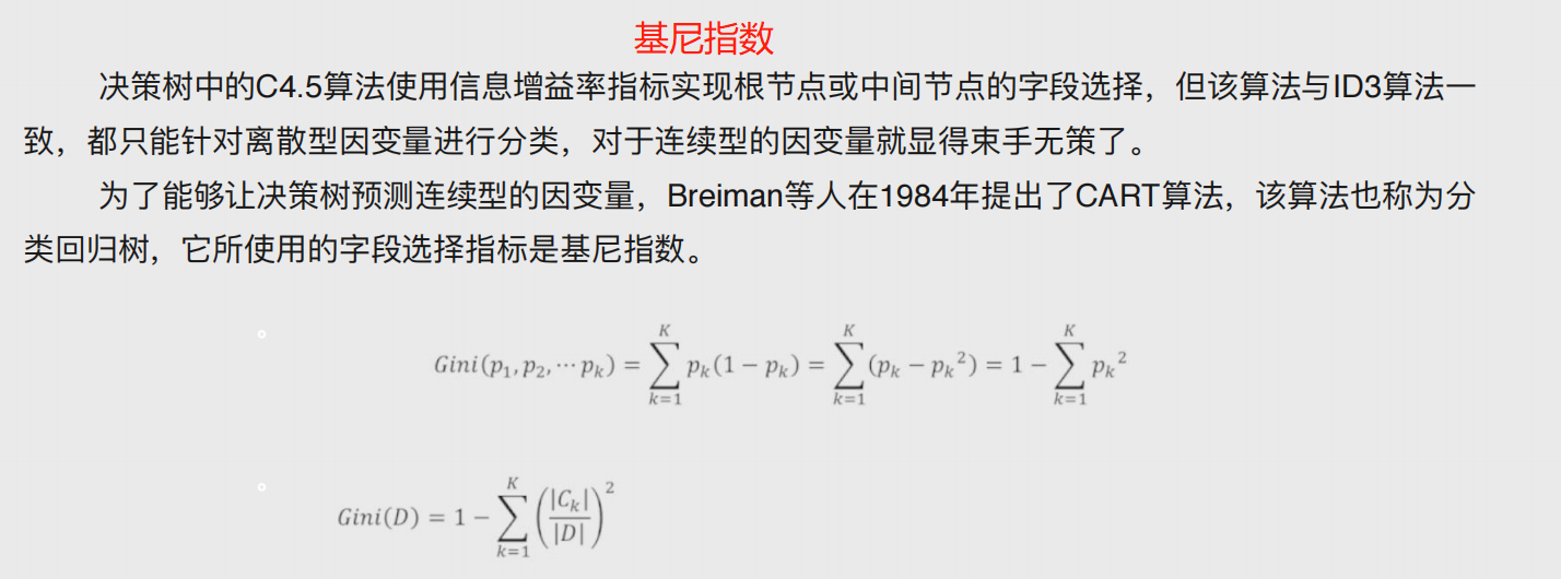
基尼指数

将模型数学化，从而能够解决连续性变量问题即预测性问题

基尼指数越小，说明数据集纯度越高，不确定性就越小，就越容易区分。

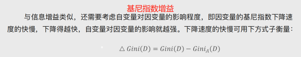
基尼指数增益

自变量对因变量的影响程度。

决策树参数说明

DecisionTreeClassifier(criterion='gini', splitter='best',
max_depth=None,min_samples_split=2,
min_samples_leaf=1,max_leaf_nodes=None,
class_weight=None)
# 参数
criterion：⽤于指定选择节点字段的评价指标，对于分类决策树，默认为'gini'，表示采⽤基尼指数选
择节点的最佳分割字段；对于回归决策树，默认为'mse'，表示使⽤均⽅误差选择节点的最佳分割字段
splitter：⽤于指定节点中的分割点选择⽅法，默认为'best'，表示从所有的分割点中选择最佳分割点；
如果指定为'random'，则表示随机选择分割点
max_depth：⽤于指定决策树的最⼤深度，默认为None，表示树的⽣⻓过程中对深度不做任何限制
min_samples_split：⽤于指定根节点或中间节点能够继续分割的最⼩样本量， 默认为2
min_samples_leaf：⽤于指定叶节点的最⼩样本量，默认为1
max_leaf_nodes：⽤于指定最⼤的叶节点个数，默认为None，表示对叶节点个数不做任何限制
class_weight：⽤于指定因变量中类别之间的权重，默认为None，表示每个类别的权重都相等；如果
为balanced，则表示类别权重与原始样本中类别的⽐例成反⽐；还可以通过字典传递类别之间的权重
差异，其形式为{class_label:weight}

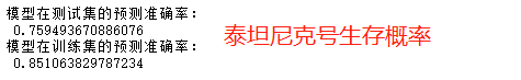
决策树案例

# 导入第三方模块
import pandas as pd
import numpy as np
import matplotlib.pyplot as plt
from sklearn import model_selection
from sklearn import linear_model
# 读⼊数据
Titanic = pd.read_csv(r'Titanic.csv')
Titanic
# 删除⽆意义的变量，并检查剩余变量是否含有缺失值
Titanic.drop(['PassengerId','Name','Ticket','Cabin'], axis = 1, inplace = True)
Titanic.isnull().sum(axis = 0)
# 对Sex分组，⽤各组乘客的平均年龄填充各组中的缺失年龄
fillna_Titanic = []
for i in Titanic.Sex.unique():
    update = Titanic.loc[Titanic.Sex == i,].fillna(value = {'Age': Titanic.Age[Titanic.Sex == i].mean()}, inplace
    = False)
fillna_Titanic.append(update)
Titanic = pd.concat(fillna_Titanic)
# 使⽤Embarked变量的众数填充缺失值
Titanic.fillna(value = {'Embarked':Titanic.Embarked.mode()[0]}, inplace=True)
​
# 将数值型的Pclass转换为类别型，否则⽆法对其哑变量处理
Titanic.Pclass = Titanic.Pclass.astype('category')
# 哑变量处理
dummy = pd.get_dummies(Titanic[['Sex','Embarked','Pclass']])
# ⽔平合并Titanic数据集和哑变量的数据集
Titanic = pd.concat([Titanic,dummy], axis = 1)
# 删除原始的Sex、Embarked和Pclass变量
Titanic.drop(['Sex','Embarked','Pclass'], inplace=True, axis = 1)
# 取出所有⾃变量名称
predictors = Titanic.columns[1:]
# 将数据集拆分为训练集和测试集，且测试集的⽐例为25%
X_train, X_test, y_train, y_test = model_selection.train_test_split(Titanic[predictors], Titanic.Survived,
test_size = 0.25, random_state = 1234)
​
from sklearn.model_selection import GridSearchCV
from sklearn import tree,metrics
# 预设各参数的不同选项值
max_depth = [2,3,4,5,6]
min_samples_split = [2,4,6,8]
min_samples_leaf = [2,4,8,10,12]
# 将各参数值以字典形式组织起来
parameters = {'max_depth':max_depth, 'min_samples_split':min_samples_split,
'min_samples_leaf':min_samples_leaf}
# ⽹格搜索法，测试不同的参数值
grid_dtcateg = GridSearchCV(estimator = tree.DecisionTreeClassifier(), param_grid = parameters, cv=10)
# 模型拟合
grid_dtcateg.fit(X_train, y_train)
# 返回最佳组合的参数值
grid_dtcateg.param_grid
​
# 构建分类决策树
CART_Class = tree.DecisionTreeClassifier(max_depth=3,min_samples_leaf=4,min_samples_split=2)
# 模型拟合
decision_tree = CART_Class.fit(X_train,y_train)
# 模型在测试集上的预测
pred = CART_Class.predict(X_test)
# 模型的准确率
print('模型在测试集的预测准确率：\n',metrics.accuracy_score(y_test,pred))
print('模型在训练集的预测准确率：\n',metrics.accuracy_score(y_train,CART_Class.predict(X_train)))

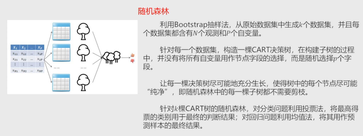
随机森林

由每颗决策树随机选择条件节点构成

对于分类问题使用投票法即选择树

对于回归问题使用均值法即求解回归模型参数

---

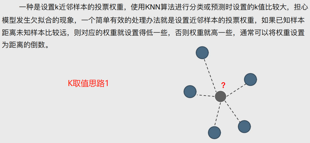
• K近邻模型

该模型既可以解决分类问题 也可以解决预测问题。

本质就是根据位置样本周边K个邻居样本做出预测。

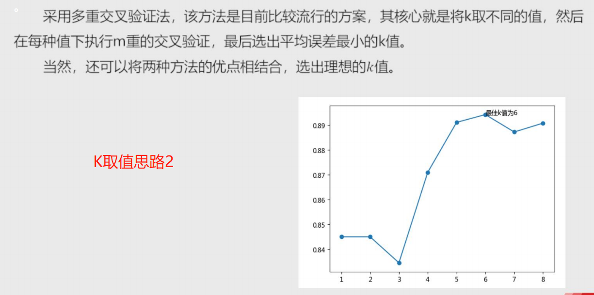
K如何取值合适？？？不能过拟合也不能欠拟合。

　　过拟合：精确度过高

　　欠拟合：精确度过低

 

 

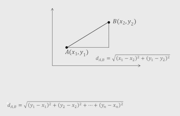
距离

1、欧氏距离：两点间直线距离。

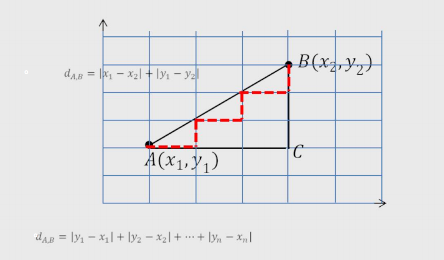
2、曼哈顿距离：两点间绕过障碍物的距离。

 

3、余弦相似度：测量两个向量的夹角的余弦值来度量它们之间的相似性，可以用于论文查重。

KNN模型参数说明

neighbors.KNeighborsClassifier(n_neighbors=5, weights='uniform',p=2, metric='minkowski',)
# 参数
n_neighbors:⽤于指定近邻样本个数K，默认为5
weights:⽤于指定近邻样本的投票权重，默认为'uniform'，表示所有近邻样本的投票权重⼀样；如果
为'distance'，则表示投票权重与距离成反⽐，即近邻样本与未知类别的样本点距离越远，权重越⼩，
反之，权重越⼤
metric:⽤于指定距离的度量指标,默认为闵可夫斯基距离
p:当参数metric为闵可夫斯基距离时,p=1,表示计算点之间的曼哈顿距离;p=2，表示计算点之间的欧⽒距离,默认值为2

KNN模型代码实现

案例1

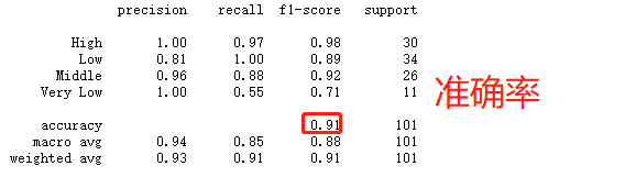
# 导入第三方包
import pandas as pd
# 导入数据
Knowledge = pd.read_excel(r'Knowledge.xlsx')
# 返回前5行数据
Knowledge.head()
# 构造训练集和测试集
# 导入第三方模块
from sklearn import model_selection
# 将数据集拆分为训练集和测试集
predictors = Knowledge.columns[:-1]
predictors
X_train, X_test, y_train, y_test = model_selection.train_test_split(Knowledge[predictors], Knowledge.UNS,test_size = 0.25, random_state = 1234)
# 导入第三方模块
import numpy as np
from sklearn import neighbors
import matplotlib.pyplot as plt
​
# 设置待测试的不同k值
K = np.arange(1,np.ceil(np.log2(Knowledge.shape[0]))).astype(int)
# 构建空的列表，用于存储平均准确率
accuracy = []
for k in K:
    # 使用10重交叉验证的方法，比对每一个k值下KNN模型的预测准确率
    cv_result = model_selection.cross_val_score(neighbors.KNeighborsClassifier(n_neighbors = k, weights = 'distance'), 
                                                X_train, y_train, cv = 10, scoring='accuracy')
    accuracy.append(cv_result.mean())
​
# 从k个平均准确率中挑选出最大值所对应的下标    
arg_max = np.array(accuracy).argmax()
# 中文和负号的正常显示
plt.rcParams['font.sans-serif'] = ['Microsoft YaHei']
plt.rcParams['axes.unicode_minus'] = False
# 绘制不同K值与平均预测准确率之间的折线图
plt.plot(K, accuracy)
# 添加点图
plt.scatter(K, accuracy)
# 添加文字说明
plt.text(K[arg_max], accuracy[arg_max], '最佳k值为%s' %int(K[arg_max]))
# 显示图形
plt.show()
​
# 导入第三方模块
from sklearn import metrics
# 重新构建模型，并将最佳的近邻个数设置为6
knn_class = neighbors.KNeighborsClassifier(n_neighbors = 6, weights = 'distance')
# 模型拟合
knn_class.fit(X_train, y_train)
# 模型在测试数据集上的预测
predict = knn_class.predict(X_test)
# 构建混淆矩阵
cm = pd.crosstab(predict,y_test)
cm
# 导入第三方模块
import seaborn as sns
​
# 将混淆矩阵构造成数据框，并加上字段名和行名称，用于行或列的含义说明
cm = pd.DataFrame(cm)
# 绘制热力图
sns.heatmap(cm, annot = True,cmap = 'GnBu')
# 添加x轴和y轴的标签
plt.xlabel(' Real Lable')
plt.ylabel(' Predict Lable')
# 图形显示
plt.show()
# 模型整体的预测准确率
metrics.scorer.accuracy_score(y_test, predict)
# 分类模型的评估报告
print(metrics.classification_report(y_test, predict))

案例2

# 读入数据
ccpp = pd.read_excel(r'CCPP.xlsx')
ccpp.head()
# 返回数据集的行数与列数
ccpp.shape
###################################################
# 导入第三方包
from sklearn.preprocessing import minmax_scale
# 对所有自变量数据作标准化处理（统一量纲）
predictors = ccpp.columns[:-1]
X = minmax_scale(ccpp[predictors])
###################################################
# 将数据集拆分为训练集和测试集
X_train, X_test, y_train, y_test = model_selection.train_test_split(X, ccpp.PE, test_size = 0.25, random_state = 1234)
# 设置待测试的不同k值
K = np.arange(1,np.ceil(np.log2(ccpp.shape[0]))).astype(int)
# 构建空的列表，用于存储平均MSE
mse = []
for k in K:
    # 使用10重交叉验证的方法，比对每一个k值下KNN模型的计算MSE
    cv_result = model_selection.cross_val_score(neighbors.KNeighborsRegressor(n_neighbors = k, weights = 'distance'), 
                                                X_train, y_train, cv = 10, scoring='neg_mean_squared_error')
    mse.append((-1*cv_result).mean())
​
# 从k个平均MSE中挑选出最小值所对应的下标  
arg_min = np.array(mse).argmin()
# 绘制不同K值与平均MSE之间的折线图
plt.plot(K, mse)
# 添加点图
plt.scatter(K, mse)
# 添加文字说明
plt.text(K[arg_min], mse[arg_min] + 0.5, '最佳k值为%s' %int(K[arg_min]))
# 显示图形
plt.show()
# 重新构建模型，并将最佳的近邻个数设置为7
knn_reg = neighbors.KNeighborsRegressor(n_neighbors = 7, weights = 'distance')
# 模型拟合
knn_reg.fit(X_train, y_train)
# 模型在测试集上的预测
predict = knn_reg.predict(X_test)
# 计算MSE值
metrics.mean_squared_error(y_test, predict)
​
# 导入第三方模块
from sklearn import tree
​
# 预设各参数的不同选项值
max_depth = [19,21,23,25,27]
min_samples_split = [2,4,6,8]
min_samples_leaf = [2,4,8,10,12]
parameters = {'max_depth':max_depth, 'min_samples_split':min_samples_split, 'min_samples_leaf':min_samples_leaf}
# 网格搜索法，测试不同的参数值
grid_dtreg = model_selection.GridSearchCV(estimator = tree.DecisionTreeRegressor(), param_grid = parameters, cv=10)
# 模型拟合
grid_dtreg.fit(X_train, y_train)
# 返回最佳组合的参数值
grid_dtreg.best_params_
# 构建用于回归的决策树
CART_Reg = tree.DecisionTreeRegressor(max_depth = 25, min_samples_leaf = 10, min_samples_split = 4)
# 回归树拟合
CART_Reg.fit(X_train, y_train)
# 模型在测试集上的预测
pred = CART_Reg.predict(X_test)
# 计算衡量模型好坏的MSE值
metrics.mean_squared_error(y_test, pred)