
目录:
2. DataFrame属性:values、columns、index、shape
五、pandas的数据处理
import pandas as pd
from pandas import Series,DataFrame
一、Pandas的数据结构
(一)、Series
Series是一种类似与一维数组的对象,由下面两个部分组成:
values:一组数据(ndarray类型)
index:相关的数据索引标签
1.Series的创建
两种创建方式:
1.1 由列表或numpy数组创建
注意:默认索引为0到N-1的整数型索引
1.1.1 #使用列表创建Series
Series(data=[1,2,3,4,5])
输出:
        0    1
        1    2
        2    3
        3    4
        4    5
        dtype: int64
1.1.2 #使用numpy创建Series
import numpy as np
Series(data=np.random.randint(1,40,size=(5,)),index=['a','d','f','g','t'],name='bobo')
输出:
        a     3
        d    22
        f    35
        g    19
        t    21
        Name: bobo, dtype: int32
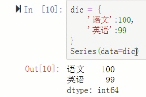
1.2 由字典创建:不能再使用index.但是依然存在默认索引
注意:数据源必须为一维数据
dic = {
'语文':100,
'英语':99
}
s = Series(data=dic)
2. Series的索引和切片
2.1 索引
可以使用中括号取单个索引(此时返回的是元素类型),或者中括号里一个列表取多个索引(此时返回的是一个Series类型)。
2.1.1 显式索引:
    - 使用index中的元素作为索引值
    - 使用s.loc[](推荐):注意,loc中括号中放置的一定是显式索引,iloc括号中放置的一定是隐式索引
注意,此时是闭区间
s.iloc[1]
输出: 99
2.1.2 隐式索引:
    - 使用整数作为索引值
    - 使用.iloc[](推荐):iloc中的中括号中必须放置隐式索引
注意,此时是半开区间
2.2 切片
2.2.1 显示索引切片:index和loc 注意,loc中括号中放置的一定是显式索引
s.iloc[0:2]
输出:
      语文    100
      英语     99
      dtype: int64
2.2.2 隐式索引切片:整数索引值和iloc iloc中的中括号中必须放置隐式索引
3. Series的基本概念
可以把Series看成一个定长的有序字典
向Series增加一行:相当于给字典增加一组键值对
3.1 可以通过shape,size,index,values等得到series的属性
3.1.1 s.index
输出:Index(['语文', '英语'], dtype='object')
3.1.2 s.values
输出:array([100, 99], dtype=int64)
3.2 可以使用s.head(),tail()分别查看前n个和后n个值
3.2.1 s.head(1)
输出:
      语文    100
      dtype: int64
3.3 对Series元素进行去重
s = Series(data=[1,1,2,2,3,3,4,4,4,4,4,5,6,7,55,55,44])
s.unique()
输出:array([ 1, 2, 3, 4, 5, 6, 7, 55, 44], dtype=int64)
3.4 数据清洗
当索引没有对应的值时,可能出现缺失数据显示NaN(not a number)的情况
3.4.1 使得两个Series进行相加:索引与之对应的元素会进行算数运算,不对应的就补空
s1 = Series([1,2,3,4,5],index=['a','b','c','d','e'])
s2 = Series([1,2,3,4,5],index=['a','b','f','c','e'])
s = s1+s2
s
输出:
      a     2.0
      b     4.0
      c     7.0
      d     NaN
      e    10.0
      f     NaN
      dtype: float64
3.4.2 可以使用pd.isnull(),pd.notnull(),或s.isnull(),notnull()函数检测缺失数据
s.notnull()
输出:
        a     True
        b     True
        c     True
        d    False
        e     True
        f    False
        dtype: bool
s[s.notnull()]
输出:
        a     2.0
        b     4.0
        c     7.0
        e    10.0
        dtype: float64
4. Series的运算
4.1 + - * /
4.2 add() sub() mul() div() : s1.add(s2,fill_value=0)
s1.add(s2)
输出:
      a     2.0
      b     4.0
      c     7.0
      d     NaN
      e    10.0
      f     NaN
       dtype: float64
4.3 Series之间的运算
在运算中自动对齐不同索引的数据
如果索引不对应,则补NaN
(二)、DataFrame
DataFrame是一个【表格型】的数据结构。DataFrame由按一定顺序排列的多列数据组成。设计初衷是将Series的使用场景从一维拓展到多维。DataFrame既有行索引,也有列索引。
行索引:index
列索引:columns
值:values
1. DataFrame的创建
注:最常用的方法是传递一个字典来创建。DataFrame以字典的键作为每一【列】的名称,以字典的值(一个数组)作为每一列。
此外,DataFrame会自动加上每一行的索引。
使用字典创建的DataFrame后,则columns参数将不可被使用。
同Series一样,若传入的列与字典的键不匹配,则相应的值为NaN。
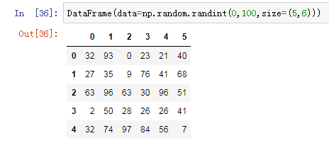
1.1 使用 ndarray 创建DataFrame
import numpy as np
DataFrame(data=np.random.randint(0,100,size=(5,6)))
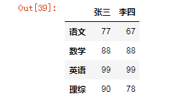
1.2 使用 字典 创建DataFrame:创建一个表格用于展示张三,李四的语文、英语、数学、理综的成绩
dic = {
'张三':[77,88,99,90],
'李四':[67,88,99,78]
}
df = DataFrame(data=dic,index=['语文','数学','英语','理综'])
df
2. DataFrame属性:values、columns、index、shape
2.1 df.values
输出:
    array([[77, 67],
           [88, 88],
           [99, 99],
           [90, 78]], dtype=int64)
2.2 df.index
输出:
Index(['语文', '数学', '英语', '理综'], dtype='object')
3. DataFrame的索引、切片


DataFrame
- 索引:
    - df[col] df[[c1,c2]]:取列
    - df.loc[index] : 取行
    - df.loc[index,col] : 取元素
- 切片:
    - df[a:b]:切行
    - df.loc[:,a:b]:切列
- df运算:Series运算一致
- df级联:拼接
3.1 对列进行索引
通过类似字典的方式 df['q']
通过属性的方式 df.q
可以将DataFrame的列获取为一个Series。返回的Series拥有原DataFrame相同的索引,且name属性也已经设置好了,就是相应的列名。
3.1.1 df['张三']
输出:
        语文    77
        数学    88
        英语    99
        理综    90
        Name: 张三, dtype: int64
3.1.2 df.张三
输出:
        语文    77
        数学    88
        英语    99
        理综    90
        Name: 张三, dtype: int64
3.1.3 df[['李四','张三']]
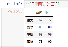
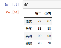
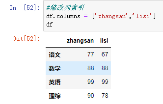
3.1.4 #修改列索引
df
3.2 对行进行索引
使用.loc[]加index来进行行索引
使用.iloc[]加整数来进行行索引
同样返回一个Series,index为原来的columns。
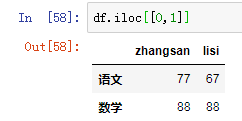
df.iloc[[0,1]]
3.3 对元素索引的方法
使用列索引
使用行索引(iloc[3,1] or loc['C','q']) 行索引在前,列索引在后
df.iloc[0,1]
输出:67
3.4 切片:
注意:直接用中括号时:
索引表示的是列索引
切片表示的是行切片
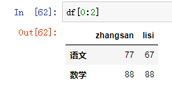
3.4.1 df[0:2]
3.4.2 在loc和iloc中使用切片(切列) : df.loc['B':'C','丙':'丁']
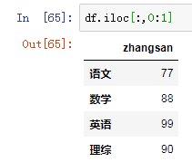
df.iloc[:,0:1]
4. DataFrame的运算
注:同Series一样:
在运算中自动对齐不同索引的数据
如果索引不对应,则补NaN
练习:
-
假设df是期中考试成绩,df2是期末考试成绩,将两者相加,求期中期末平均值。
-
假设张三期中考试数学被发现作弊,要记为0分,如何实现?
-
李四因为举报张三作弊立功,期中考试所有科目加100分,如何实现?
-
后来老师发现期中考试有一道题出错了,为了安抚学生情绪,给每位学生期中考试每个科目都加10分,如何实现?
答案:
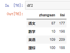
1. (df+df2)/2
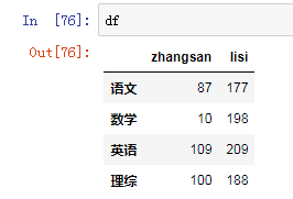
2. df.loc['数学','zhangsan'] = 0
3. df['lisi'] += 100
4. df += 10
import tushare as ts
import pandas as pd
from pandas import DataFrame,Series

df = ts.get_k_data('600519',start='1999-01-01')   # 获取茅台股票自开售之日到今天的所有信息,600519为茅台股票代码

#将df存储到本地
df.to_csv('./maotai.csv')

#将date这列数据类型转成时间序列,然后将该列作为原数据的行索引
df = pd.read_csv('./maotai.csv',index_col='date',parse_dates=['date'])    # parse_dates=['date'] 可以将date这列数据类型转成时间序列, index_col='date' 将时间列作为原数据的行索引
df.drop(labels='Unnamed: 0',axis=1,inplace=True)   # labels='Unnamed: 0',axis=1 表示不显示没用的那行;inplace=True 表示作用到原数据上
df.head(5)  # 显示前5行

    date      open      close      high        low          volume      code

2001-08-27    5.392    5.554    5.902    5.132    406318.00    600519
2001-08-28    5.467    5.759    5.781    5.407    129647.79    600519
2001-08-29    5.777    5.684    5.781    5.640    53252.75    600519
2001-08-30    5.668    5.796    5.860    5.624    48013.06    600519
2001-08-31    5.804    5.782    5.877    5.749    23231.48    600519


#输出该股票所有收盘比开盘上涨3%以上的日期。
s = (df['close'] - df['open'])/df['open'] > 0.03
df.loc[s].index

输出:DatetimeIndex(['2001-08-27', '2001-08-28', '2001-09-10', '2001-12-21',
               '2002-01-18', '2002-01-31', '2003-01-14', '2003-10-29',
               '2004-01-05', '2004-01-14',
               ...
               '2018-08-27', '2018-09-18', '2018-09-26', '2018-10-19',
               '2018-10-31', '2018-11-13', '2018-12-28', '2019-01-15',
               '2019-02-11', '2019-03-01'],
              dtype='datetime64[ns]', name='date', length=294, freq=None)


#输出该股票所有开盘比前日收盘跌幅超过2%的日期。
s1 = (df['open'] - df['close'].shift(1))/df['close'].shift(1) < -0.02
df.loc[s1].index


#假如我从2010年1月1日开始,每月第一个交易日买入1手股票,每年最后一个交易日卖出所有股票,到今天为止,我的收益如何?
price_last = df['open'][-1]
df = df['2010':'2019'] #剔除首尾无用的数据
#Pandas提供了resample函数用便捷的方式对时间序列进行重采样,根据时间粒度的变大或者变小分为降采样和升采样:
df_monthly = df.resample("M").first()
df_yearly = df.resample("Y").last()[:-1] #去除最后一年
cost_money = 0
hold = 0 #每年持有的股票
for year in range(2010, 2020):

    cost_money -= df_monthly.loc[str(year)]['open'].sum()*100
    hold += len(df_monthly[str(year)]['open']) * 100
    if year != 2019:
        cost_money += df_yearly[str(year)]['open'][0] * hold
        hold = 0 #每年持有的股票
cost_money += hold * price_last

print(cost_money)    # 310250.69999999984
二、处理丢失数据(数据清洗)
有两种丢失数据:
None:None是Python自带的,其类型为python object。因此,None不能参与到任何计算中。
np.nan(NaN):np.nan是浮点类型,能参与到计算中。但计算的结果总是NaN
pandas中的None与NaN
import numpy as np
import pandas as pd
from pandas import Series,DataFrame
1、pandas中None与np.nan都视作np.nan
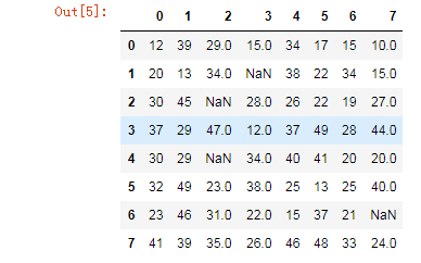
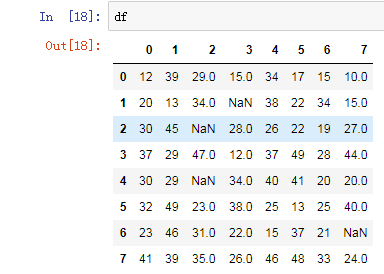
1.1 创建DataFrame
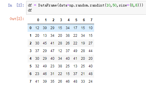
df = DataFrame(data=np.random.randint(10,50,size=(8,8)))
df
1.2 #将某些数组元素赋值为nan
df.iloc[1,3] = None
df.iloc[2,2] = None
df.iloc[4,2] = None
df.iloc[6,7] = np.nan
df
2、pandas处理空值操作
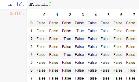
isnull()
notnull()
dropna(): 过滤丢失数据
fillna(): 填充丢失数据
2.1 判断函数(isnull()、notnull())
注: notnull配合all isnull配合any
df.isnull()
#创建DataFrame,给其中某些元素赋值为nan
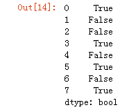
df.notnull().all(axis=1) # notnull配合all isnull配合any
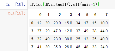
#过滤df中的空值(只保留没有空值的行)
df.loc[df.notnull().all(axis=1)]
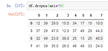
2.2 过滤函数
df.dropna() 可以选择过滤的是行还是列(默认为行):axis中0表示行,1表示的列
df.dropna(axis=0)
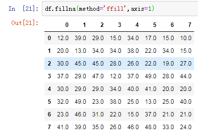
2.3 填充函数
fillna():value和method参数
注:可以选择前向填充还是后向填充;method 控制填充的方式 ffill bfill
df.fillna(method='ffill',axis=1)
三、多层索引
1. 创建多层列索引
1.1 隐式构造
最常见的方法是给DataFrame构造函数的index或者columns参数传递两个或更多的数组
1.2 显示构造pd.MultiIndex.from_
1.2.1 使用数组
1.2.2 使用product (最简单,推荐使用)
import numpy as np
import pandas as pd
from pandas import Series,DataFrame
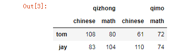
col=pd.MultiIndex.from_product([['qizhong','qimo'],['chinese','math']])
# 创建DF对象
df = DataFrame(data=np.random.randint(60,120,size=(2,4)),index=['tom','jay'],
columns=col)
df
df['qimo']

2. 多层行索引
除了列索引,行索引也能用上述同样的方法创建多层行索引
3. 多层索引对象的索引与切片操作
注意在对行索引的时候,若一级行索引还有多个,对二级行索引会遇到问题!也就是说,无法直接对二级索引进行索引,必须让二级索引变成一级索引后才能对其进行索引!
# 总结:
# 访问一列或多列 直接用中括号[columnname] [[columname1,columnname2...]]
# 访问一行或多行 .loc[indexname]
# 访问某一个元素 .loc[indexname,columnname] 获取李四期中的php成绩
# 行切片 .loc[index1:index2] 获取张三李四的期中成绩
# 列切片 .loc[:,column1:column2] 获取张三李四期中的php和c++成绩
4. 聚合操作
所谓的聚合操作:平均数,方差,最大值,最小值……
四、pandas的拼接操作
pandas的拼接分为两种:
级联:pd.concat, pd.append
合并:pd.merge, pd.join
import numpy as np
import pandas as pd
from pandas import Series,DataFrame
1. 使用pd.concat()级联
pandas使用pd.concat函数,与np.concatenate函数类似,只是多了一些参数:
objs
axis=0
keys
join='outer' / 'inner':表示的是级联的方式,outer会将所有的项进行级联(忽略匹配和不匹配),而inner只会将匹配的项级联到一起,不匹配的不级联
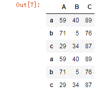
ignore_index=Falsedf1 = DataFrame(data=np.random.randint(0,100,size=(3,3)),index=['a','b','c'],columns=['A','B','C'])
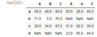
df2 = DataFrame(data=np.random.randint(0,100,size=(3,3)),index=['a','d','c'],columns=['A','d','C'])
1.1 匹配级联
pd.concat((df1,df1),axis=0,join='inner')
1.2 不匹配级联
不匹配指的是级联的维度的索引不一致。例如纵向级联时列索引不一致,横向级联时行索引不一致
有2种连接方式:
外连接:补NaN(默认模式)
内连接:只连接匹配的项
pd.concat((df1,df2),axis=1,join='outer')
1.3 使用df.append()函数添加
由于在后面级联的使用非常普遍,因此有一个函数append专门用于在后面添加
2. 使用pd.merge()合并
merge与concat的区别在于,merge需要依据某一共同的列来进行合并
使用pd.merge()合并时,会自动根据两者相同column名称的那一列,作为key来进行合并。
注意每一列元素的顺序不要求一致
参数:
how:out取并集 inner取交集
on:当有多列相同的时候,可以使用on来指定使用那一列进行合并,on的值为一个列表
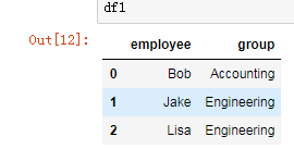
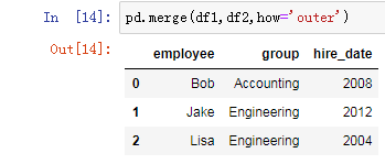
2.1 一对一合并
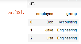
df1 = DataFrame({'employee':['Bob','Jake','Lisa'],
'group':['Accounting','Engineering','Engineering'],
})
df1
df2 = DataFrame({'employee':['Lisa','Bob','Jake'],
'hire_date':[2004,2008,2012],
})
df2
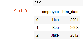
pd.merge(df1,df2,how='outer')
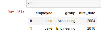
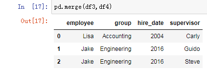
2.2 多对一合并
df3 = DataFrame({
'employee':['Lisa','Jake'],
'group':['Accounting','Engineering'],
'hire_date':[2004,2016]})
df3
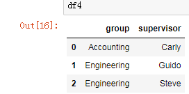
df4 = DataFrame({'group':['Accounting','Engineering','Engineering'],
'supervisor':['Carly','Guido','Steve']
})
df4
pd.merge(df3,df4)
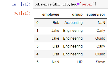
2.3 多对多合并
df1 = DataFrame({'employee':['Bob','Jake','Lisa'],
'group':['Accounting','Engineering','Engineering']})
df1
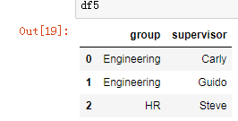
df5 = DataFrame({'group':['Engineering','Engineering','HR'],
'supervisor':['Carly','Guido','Steve']
})
df5
pd.merge(df1,df5,how='outer')
注:加载excl数据:pd.read_excel('excl_path',sheetname=1)
2.4 key的规范化
当列冲突时,即有多个列名称相同时,需要使用on=来指定哪一个列作为key,配合suffixes指定冲突列名
当两张表没有可进行连接的列时,可使用left_on和right_on手动指定merge中左右两边的哪一列列作为连接的列
2.5 内合并与外合并:out取并集 inner取交集
内合并:只保留两者都有的key(默认模式)
外合并 how='outer':补NaN
需求:
    1. 导入文件,查看原始数据
    2. 将人口数据和各州简称数据进行合并
    3. 将合并的数据中重复的abbreviation列进行删除
    4. 查看存在缺失数据的列
    5. 找到有哪些state/region使得state的值为NaN,进行去重操作
    6. 为找到的这些state/region的state项补上正确的值,从而去除掉state这一列的所有NaN
    7. 合并各州面积数据areas
    8. 我们会发现area(sq.mi)这一列有缺失数据,找出是哪些行
    9. 去除含有缺失数据的行
    10. 找出2010年的全民人口数据
    11. 计算各州的人口密度
    12. 排序,并找出人口密度最高的五个州 df.sort_values()


import numpy as np
from pandas import DataFrame,Series
import pandas as pd

1. 导入文件,查看原始数据
    abb = pd.read_csv('./data/state-abbrevs.csv')   # 各州简称
    pop = pd.read_csv('./data/state-population.csv')   # 人口数据
    area = pd.read_csv('./data/state-areas.csv')    # 各州面积

2. 将人口数据和各州简称数据进行合并
    abb_pop = pd.merge(abb,pop,left_on='abbreviation',right_on='state/region',how='outer')
    abb_pop.head()

    state       abbreviation    state/region    ages    year    population
    0    Alabama    AL    AL    under18    2012    1117489.0
    1    Alabama    AL    AL    total    2012    4817528.0
    2    Alabama    AL    AL    under18    2010    1130966.0
    3    Alabama    AL    AL    total    2010    4785570.0
    4    Alabama    AL    AL    under18    2011    1125763.0

3. 将合并的数据中重复的abbreviation列进行删除
    abb_pop.drop(labels='abbreviation',axis=1,inplace=True)

4. 查看存在缺失数据的列
    abb_pop.isnull().any(axis=0)
    输出:
             state            True
           state/region    False
           ages            False
           year            False
           population       True
           dtype: bool

5. 找到有哪些state/region使得state的值为NaN,进行去重操作
     #1.检测state列中的空值
          abb_pop['state'].isnull()
     #2.将1的返回值作用到state_region这一列中
          abb_pop['state/region'][abb_pop['state'].isnull()]
     #3.去重
          abb_pop['state/region'][abb_pop['state'].isnull()].unique()
     输出:array(['PR','USA'], dtype=object)

6. 为找到的这些state/region的state项补上正确的值,从而去除掉state这一列的所有NaN
    usa_indexs = abb_pop['state'][abb_pop['state/region'] == 'USA'].index
    abb_pop.loc[usa_indexs,'state'] = 'United State'
    pr_indexs = abb_pop['state'][abb_pop['state/region'] == 'PR'].index
    abb_pop.loc[pr_indexs,'state'] = 'PPPRRR'

7. 合并各州面积数据areas
    abb_pop_area = pd.merge(abb_pop,area,how='outer')
    abb_pop_area.head()
    输出:
            state    state/region    ages    year    population    area (sq. mi)
    0     Alabama      AL     under18     2012.0    1117489.0    52423.0
    1     Alabama      AL     total     2012.0    4817528.0    52423.0
    2     Alabama      AL     under18     2010.0    1130966.0    52423.0
    3     Alabama      AL     total     2010.0    4785570.0    52423.0
    4     Alabama      AL     under18     2011.0    1125763.0    52423.0

8. 我们会发现area(sq.mi)这一列有缺失数据,找出是哪些行
    n = abb_pop_area['area (sq. mi)'].isnull()
    a_index = abb_pop_area.loc[n].index

9. 去除含有缺失数据的行
    abb_pop_area.drop(labels=a_index,axis=0,inplace=True)

10. 找出2010年的全民人口数据
    abb_pop_area.query('year == 2010 & ages == "total"')

11. 计算各州的人口密度
    abb_pop_area['midu'] = abb_pop_area['population'] / abb_pop_area['area (sq. mi)']

12. 排序,并找出人口密度最高的五个州 df.sort_values()
    abb_pop_area.sort_values(by='midu',axis=0,ascending=False).head()
五、pandas数据处理
1、删除重复元素
1.1 使用duplicated()函数检测重复的行,返回元素为布尔类型的Series对象,每个元素对应一行,如果该行不是第一次出现,则元素为True
keep参数:指定保留哪一重复的行数据创建具有重复元素行的DataFrame
import numpy as np
import pandas as pd
from pandas import Series,DataFrame
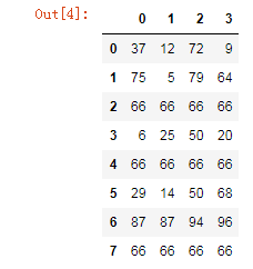
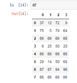
#创建一个df
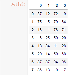
np.random.seed(1)
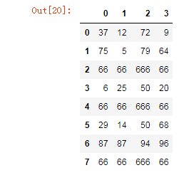
df = DataFrame(data=np.random.randint(0,100,size=(8,4)))
df
#手动将df的某几行设置成相同的内容
df.iloc[2] = [66,66,66,66]
df.iloc[4] = [66,66,66,66]
df.iloc[7] = [66,66,66,66]
df
使用duplicated查看所有重复元素行
df.duplicated(keep='last')
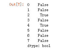
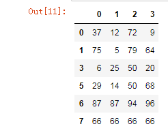
indexs = df.loc[df.duplicated(keep='last')].index
删除重复元素的行
df.drop(labels=indexs,axis=0)
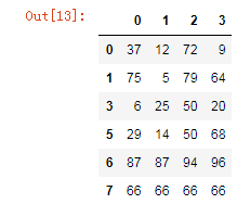
1.2 使用drop_duplicates()函数删除重复的行
drop_duplicates(keep='first/last'/False)
df.drop_duplicates(keep='last')
2. 映射
2.1 replace()函数:替换元素
使用replace()函数,对values进行映射操作
Series替换操作
-
- 单值替换
- 普通替换
- 字典替换(推荐)
- 多值替换
- 列表替换
- 字典替换(推荐)
- 参数
- to_replace:被替换的元素
- 单值替换
replace参数说明:
-
- method:对指定的值使用相邻的值填充替换
- limit:设定填充次数
DataFrame替换操作
-
- 单值替换
- 普通替换: 替换所有符合要求的元素:to_replace=15,value='e'
- 按列指定单值替换: to_replace={列标签:替换值} value='value'
- 单值替换
-
- 多值替换
- 列表替换: to_replace=[] value=[]
- 字典替换(推荐) to_replace={to_replace:value,to_replace:value}
- 多值替换
注意:DataFrame中,无法使用method和limit参数
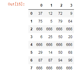
# 单值替换(普通替换)
df.replace(to_replace=66,value=666)
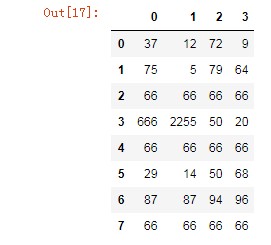
# 多值替换(列表替换)
df.replace(to_replace=[6,25],value=[666,2255])
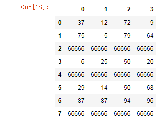
# 单值替换
df.replace(to_replace={66:66666})
# 单值替换(按列指定单值替换)
df.replace(to_replace={2:66},value=666)
2.2 map()函数:新建一列 , map函数并不是df的方法,而是series的方法
-
map()可以映射新一列数据
-
map()中可以使用lambd表达式
-
map()中可以使用方法,可以是自定义的方法
eg:map({to_replace:value})
-
注意 map()中不能使用sum之类的函数,for循环
新增一列:给df中,添加一列,该列的值为英文名对应的中文名
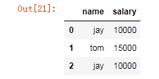
dic = {
'name':['jay','tom','jay'],
'salary':[10000,15000,10000]
}
df = DataFrame(data=dic)
df
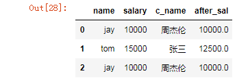
# 定制一个映射关系表
dic = {
'jay':'周杰伦',
'tom':'张三'
}
# 添加一列,该列的值为英文名对应的中文名
df['c_name'] = df['name'].map(dic)
df
map当做一种运算工具,至于执行何种运算,是由map函数的参数决定的(参数:lambda,函数)
使用自定义函数
def after_sal(s):
if s < 10000:
return s
else:
return s-(s-10000)*0.5
#超过10000部分的钱缴纳50%的税
df['after_sal'] = df['salary'].map(after_sal)
df
注意:并不是任何形式的函数都可以作为map的参数。只有当一个函数具有一个参数且有返回值,那么该函数才可以作为map的参数
3. 使用聚合操作对数据异常值检测和过滤
使用df.std()函数可以求得DataFrame对象每一列的标准差
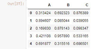
# 创建一个1000行3列的df 范围(0-1),求其每一列的标准差
df = DataFrame(data=np.random.random(size=(1000,3)),columns=['A','B','C'])
df
# 对df应用筛选条件,去除标准差太大的数据:假设过滤条件为 C列数据大于两倍的C列标准差
value_std = df['C'].std()*2
df['C'] <= value_std
df.loc[df['C'] <= value_std]
4. 排序
4.1 使用.take()函数排序
    - take()函数接受一个索引列表,用数字表示,使得df根据列表中索引的顺序进行排序
    - eg:df.take([1,3,4,2,5])
4.1.1 可以借助np.random.permutation()函数随机排序
df.head()
random_df = df.take(np.random.permutation(1000),axis=0).take(np.random.permutation(3),axis=1)
random_df[0:100]
4.1.2 np.random.permutation(x)可以生成x个从0-(x-1)的随机数列
np.random.permutation(1000)
输出:array([4, 0, 3, 2, 1])
4.2 随机抽样
当DataFrame规模足够大时,直接使用np.random.permutation(x)函数,就配合take()函数实现随机抽样
5. 数据分类处理【重点】
数据聚合是数据处理的最后一步,通常是要使每一个数组生成一个单一的数值。
数据分类处理:
-
- 分组:先把数据分为几组
- 用函数处理:为不同组的数据应用不同的函数以转换数据
- 合并:把不同组得到的结果合并起来
数据分类处理的核心:
     - groupby()函数
     - groups属性查看分组情况
     - eg: df.groupby(by='item').groups
5.1 分组
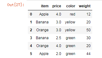
from pandas import DataFrame,Series
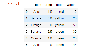
df = DataFrame({'item':['Apple','Banana','Orange','Banana','Orange','Apple'],
'price':[4,3,3,2.5,4,2],
'color':['red','yellow','yellow','green','green','green'],
'weight':[12,20,50,30,20,44]})
df
5.1.1 使用groupby实现分组
df.groupby(by='item',axis=0)
输出:<pandas.core.groupby.groupby.DataFrameGroupBy object at 0x0000000007C86208>
5.1.2 使用groups查看分组情况
#该函数可以进行数据的分组,但是不显示分组情况
df.groupby(by='item',axis=0).groups
    输出:{'Apple': Int64Index([0, 5], dtype='int64'),
        'Banana': Int64Index([1, 3], dtype='int64'),
        'Orange': Int64Index([2, 4], dtype='int64')}
5.2 分组后的聚合操作:分组后的成员中可以被进行运算的值会进行运算,不能被运算的值不进行运算
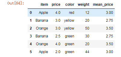
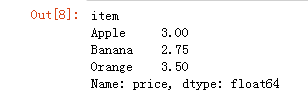
# 给df创建一个新列,内容为各个水果的平均价格
df.groupby(by='item').mean()['price']
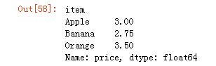
mean_price = df.groupby(by='item')['price'].mean()
dic = mean_price.to_dict()
df['mean_price'] = df['item'].map(dic)
df
# 计算出苹果的平均价格
df.groupby(by='item',axis=0).mean()['price'][0]
输出:3.0
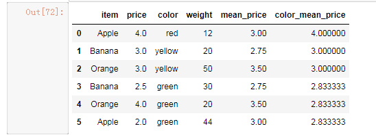
# 按颜色查看各种颜色的水果的平均价格
color_price = df.groupby(by='color')['price'].mean()
dic = color_price.to_dict()
df['color_mean_price'] = df['color'].map(dic)
df
6. 高级数据聚合
使用groupby分组后,也可以使用transform和apply提供自定义函数实现更多的运算
-
- df.groupby('item')['price'].sum() <==> df.groupby('item')['price'].apply(sum)
- transform和apply都会进行运算,在transform或者apply中传入函数即可
- transform和apply也可以传入一个lambda表达式
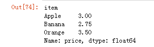
df.groupby(by='item')['price'].mean()
# 求出各种水果价格的平均值
df.groupby(by='item')['price']
输出:<pandas.core.groupby.groupby.SeriesGroupBy object at 0x1148c30f0>
df
#使用apply函数求出水果的平均价格
df.groupby(by='item')['price'].apply(fun)
def fun(s):
sum = 0
for i in s:
sum+=i
return sum/s.size
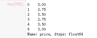
# 使用transform函数求出水果的平均价格
df.groupby(by='item')['price'].transform(fun)
方便大家操作,将月份和参选人以及所在政党进行定义:
months = {'JAN' : 1, 'FEB' : 2, 'MAR' : 3, 'APR' : 4, 'MAY' : 5, 'JUN' : 6,
          'JUL' : 7, 'AUG' : 8, 'SEP' : 9, 'OCT': 10, 'NOV': 11, 'DEC' : 12}
of_interest = ['Obama, Barack', 'Romney, Mitt', 'Santorum, Rick',
               'Paul, Ron', 'Gingrich, Newt']
parties = {
  'Bachmann, Michelle': 'Republican',
  'Romney, Mitt': 'Republican',
  'Obama, Barack': 'Democrat',
  "Roemer, Charles E. 'Buddy' III": 'Reform',
  'Pawlenty, Timothy': 'Republican',
  'Johnson, Gary Earl': 'Libertarian',
  'Paul, Ron': 'Republican',
  'Santorum, Rick': 'Republican',
  'Cain, Herman': 'Republican',
  'Gingrich, Newt': 'Republican',
  'McCotter, Thaddeus G': 'Republican',
  'Huntsman, Jon': 'Republican',
  'Perry, Rick': 'Republican'
 }

 1.读取文件usa_election.txt

 2.查看文件样式及基本信息

 3.【知识点】使用map函数+字典,新建一列各个候选人所在党派party

 4.使用np.unique()函数查看colums:party这一列中有哪些元素

 5.使用value_counts()函数,统计party列中各个元素出现次数,value_counts()是Series中的,无参,返回一个带有每个元素出现次数的Series

 6.【知识点】使用groupby()函数,查看各个党派收到的政治献金总数contb_receipt_amt

 7.查看具体每天各个党派收到的政治献金总数contb_receipt_amt 。使用groupby([多个分组参数])

 8. 将表中日期格式转换为'yyyy-mm-dd'。日期格式,通过函数加map方式进行转换

 9.查看老兵(捐献者职业)DISABLED VETERAN主要支持谁  :查看老兵们捐赠给谁的钱最多

 10.找出候选人的捐赠者中,捐赠金额最大的人的职业以及捐献额  .通过query("查询条件来查找捐献人职业")


import numpy as np
import pandas as pd
from pandas import Series,DataFrame

1、读取文件
     table = pd.read_csv('data/usa_election.txt')
     table.head()

3、使用map函数+字典,新建一列各个候选人所在党派party
     table['party'] = table['cand_nm'].map(parties)
     table.head()

4、party这一列中有哪些元素
     table['party'].unique()
     输出:array(['Republican', 'Democrat', 'Reform', 'Libertarian'], dtype=object)

5、使用value_counts()函数,统计party列中各个元素出现次数,value_counts()是Series中的,无参,返回一个带有每个元素出现次数的Series
     table['party'].value_counts()

6、使用groupby()函数,查看各个党派收到的政治献金总数contb_receipt_amt
     table.groupby(by='party')['contb_receipt_amt'].sum()

7、查看具体每天各个党派收到的政治献金总数contb_receipt_amt 。使用groupby([多个分组参数])
     table.groupby(by=['party','contb_receipt_dt'])['contb_receipt_amt'].sum()

8、将表中日期格式转换为'yyyy-mm-dd'。日期格式,通过函数加map方式进行转换
     def trasform_date(d):
          day,month,year = d.split('-')
          month = months[month]
          return "20"+year+'-'+str(month)+'-'+day
     table['contb_receipt_dt'] = table['contb_receipt_dt'].apply(trasform_date)

9、查看老兵(捐献者职业)DISABLED VETERAN主要支持谁  :查看老兵们捐赠给谁的钱最多
     old_bing_df = table.loc[table['contbr_occupation'] == 'DISABLED VETERAN']
     old_bing_df.groupby(by='cand_nm')['contb_receipt_amt'].sum()

10、找出候选人的捐赠者中,捐赠金额最大的人的职业以及捐献额  .通过query("查询条件来查找捐献人职业")
     table['contb_receipt_amt'].max()  # 1944042.43
     table.query('contb_receipt_amt == 1944042.43')
如果我从假如我从2010年1月1日开始,初始资金为100000元,金叉尽量买入,死叉全部卖出,则到今天为止,我的炒股收益率如何?

import tushare as ts
import pandas as pd
from pandas import DataFrame,Series

df = pd.read_csv('maotai.csv',index_col='date',parse_dates=['date'])
df.drop(labels='Unnamed: 0',axis=1,inplace=True)
df = df['2010':'2019']

df['ma5']=df['close'].rolling(5).mean()   # 5日均线
df['ma30']=df['close'].rolling(30).mean()   # 30日均线

sr1 = df['ma5'] < df['ma30']
sr2 = df['ma5'] >= df['ma30']
death_cross = df[sr1 & sr2.shift(1)].index    # 死叉对应日期
golden_cross = df[~(sr1 | sr2.shift(1))].index    # 金叉对应日期

first_money = 100000
money = first_money
hold = 0   # 持有多少股
sr1 = pd.Series(1, index=golden_cross)
sr2 = pd.Series(0, index=death_cross)
#根据时间排序
sr = sr1.append(sr2).sort_index()

for i in range(0, len(sr)):
    p = df['open'][sr.index[i]]
    if sr[i] == 1:
        #金叉
        buy = (money // (100 * p))
        hold += buy*100   # 持有股票数
        money -= buy*100*p
    else:
        money += hold * p
        hold = 0

p = df['open'][-1]
now_money = hold * p + money

print(now_money - first_money)    # 1086009.8999999994

 浙公网安备 33010602011771号