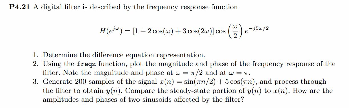
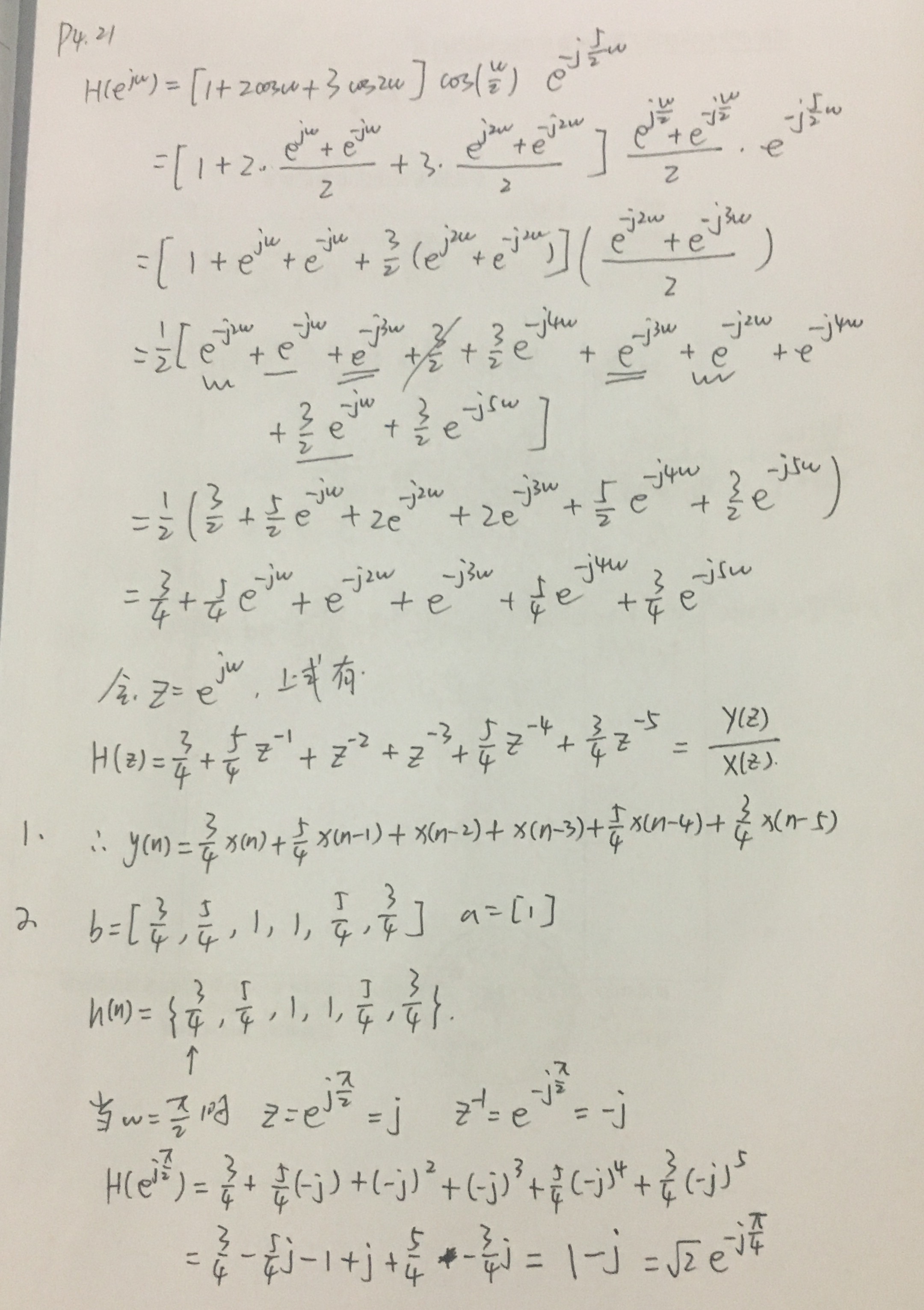
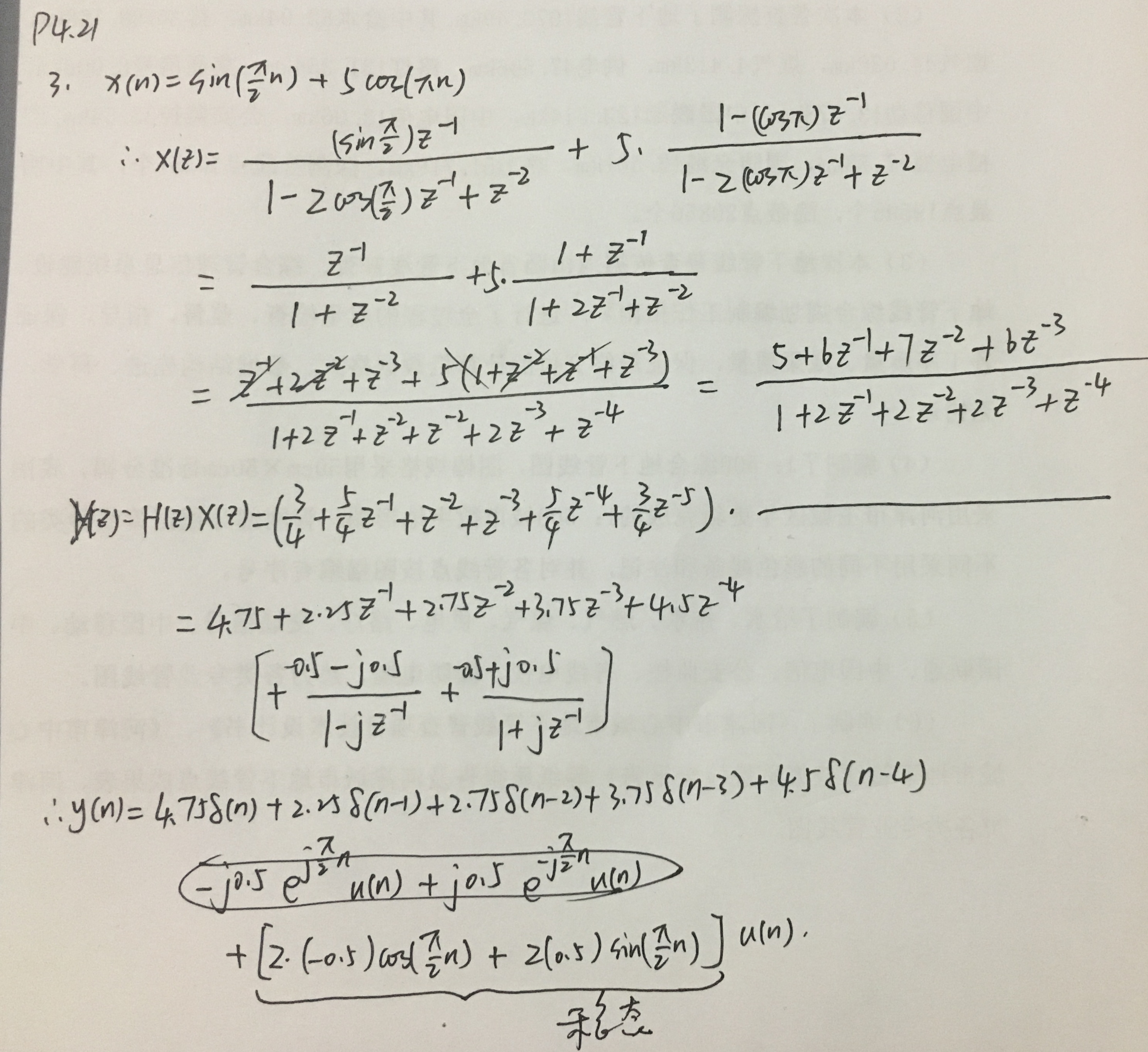
《DSP using MATLAB》Problem 4.21

        快到龙抬头，居然下雪了，天空飘起了雪花，温度下降了近20°。

代码：

%% ------------------------------------------------------------------------
%%            Output Info about this m-file
fprintf('\n***********************************************************\n');
fprintf('        <DSP using MATLAB> Problem 4.21 \n\n');

banner();
%% ------------------------------------------------------------------------


% ----------------------------------------------------
%               1        H1(z)
% ----------------------------------------------------

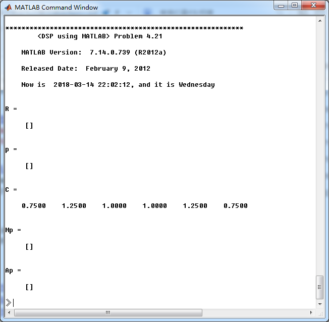
b = [3/4, 5/4, 1, 1, 5/4, 3/4]; a = [1];                             %  

[R, p, C] = residuez(b,a)

Mp = (abs(p))'
Ap = (angle(p))'/pi

%% ------------------------------------------------------
%%   START a    determine H(z) and sketch    
%% ------------------------------------------------------
figure('NumberTitle', 'off', 'Name', 'P4.21 H(z) its pole-zero plot')
set(gcf,'Color','white'); 
zplane(b,a);
title('pole-zero plot'); grid on;

%% ----------------------------------------------
%%    END
%% ----------------------------------------------

% ------------------------------------
%                  h(n)  
% ------------------------------------

[delta, n] = impseq(0, 0, 19); 
h_check = filter(b, a, delta);                                             % check sequence


%% --------------------------------------------------------------
%%    START    b   |H|   <H
%%    3rd form of freqz
%% --------------------------------------------------------------
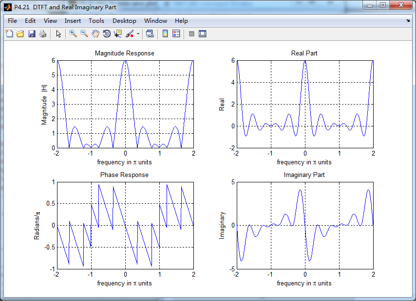
w = [-500:1:500]*2*pi/500;     H = freqz(b,a,w); 
%[H,w] = freqz(b,a,200,'whole');                 % 3rd form of freqz

magH  = abs(H);  angH  = angle(H);  realH  = real(H);  imagH  = imag(H);

%% ================================================
%%              START H's  mag ang real imag
%% ================================================
figure('NumberTitle', 'off', 'Name', 'P4.21  DTFT and Real Imaginary Part ');
set(gcf,'Color','white'); 
subplot(2,2,1); plot(w/pi,magH); grid on;  %axis([0,1,0,1.5]); 
title('Magnitude Response');
xlabel('frequency in \pi units'); ylabel('Magnitude  |H|'); 
subplot(2,2,3); plot(w/pi, angH/pi); grid on; % axis([-1,1,-1,1]);
title('Phase Response');
xlabel('frequency in \pi units'); ylabel('Radians/\pi');

subplot('2,2,2'); plot(w/pi, realH); grid on;
title('Real Part');
xlabel('frequency in \pi units'); ylabel('Real');
subplot('2,2,4'); plot(w/pi, imagH); grid on;
title('Imaginary Part');
xlabel('frequency in \pi units'); ylabel('Imaginary');
%% ==================================================
%%             END H's  mag ang real imag
%% ==================================================



% --------------------------------------------------------------
%        x(n) through the filter, we get output y(n)
% --------------------------------------------------------------
N = 200;
nx = [0:1:N-1];
 x = sin(pi*nx/2) + 5 * cos(pi*nx);

[y, ny] = conv_m(h_check, n, x, nx);

figure('NumberTitle', 'off', 'Name', 'P4.21  Input & h(n) Sequence');
set(gcf,'Color','white'); 
subplot(3,1,1); stem(nx, x); grid on;  %axis([0,1,0,1.5]); 
title('x(n)');
xlabel('n'); ylabel('x'); 
subplot(3,1,2); stem(n, h_check); grid on;  %axis([0,1,0,1.5]); 
title('h(n)');
xlabel('n'); ylabel('h'); 
subplot(3,1,3); stem(ny, y); grid on;  %axis([0,1,0,1.5]); 
title('y(n)');
xlabel('n'); ylabel('y');

figure('NumberTitle', 'off', 'Name', 'P4.21  Output Sequence');
set(gcf,'Color','white'); 
subplot(1,1,1); stem(ny, y); grid on;  %axis([0,1,0,1.5]); 
title('y(n)');
xlabel('n'); ylabel('y'); 


% ----------------------------------------
%                yss Response
% ----------------------------------------
ax = conv([1,0,1], [1,2,1])
bx = conv([0,1], [1,2,1]) + conv([5,5], [1,0,1])

by = conv(bx, b) 
ay = ax

zeros = roots(by)

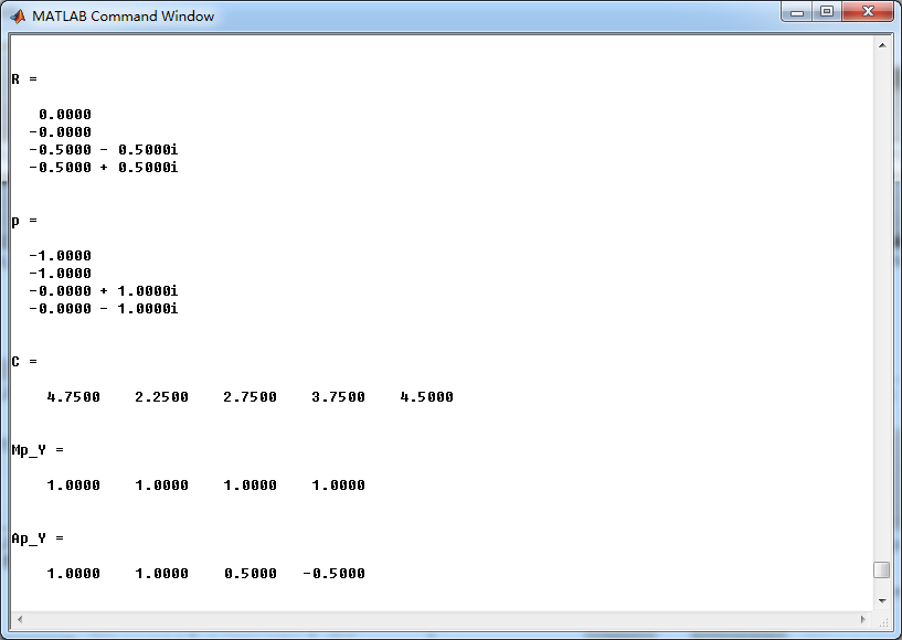
[R, p, C] = residuez(by, ay)

Mp_Y = (abs(p))'
Ap_Y = (angle(p))'/pi

%% ------------------------------------------------------
%%   START a    determine Y(z) and sketch    
%% ------------------------------------------------------
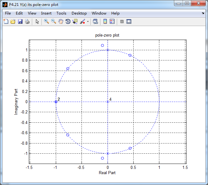
figure('NumberTitle', 'off', 'Name', 'P4.21 Y(z) its pole-zero plot')
set(gcf,'Color','white'); 
zplane(by, ay);
title('pole-zero plot'); grid on;


% ------------------------------------
%                  y(n)  
% ------------------------------------
LENGH = 100;
[delta, n] = impseq(0, 0, LENGH-1); 
y_check = filter(by, ay, delta);                                             % check sequence

y_answer0 = 4.75*delta;

[delta_1, n1] = sigshift(delta, n, 1);
y_answer1 = 2.25*delta_1;

[delta_2, n2] = sigshift(delta, n, 2);
y_answer2 = 2.75*delta_2;

[delta_3, n3] = sigshift(delta, n, 3);
y_answer3 = 3.75*delta_3; 

[delta_4, n4] = sigshift(delta, n, 4);
y_answer4 = 4.50*delta_4;

y_answer5 = (2*(-0.5)*cos(pi*n/2) + 2*0.5*sin(pi*n/2) ).*stepseq(0,0,LENGH-1);


[y01, n01] = sigadd(y_answer0, n,  y_answer1, n1);
[y02, n02] = sigadd(y_answer2, n2, y_answer3, n3);

[y03, n03] = sigadd(y01, n01, y02, n02);
[y04, n04] = sigadd(y03, n03, y_answer4, n4);

[y_answer, n_answer] = sigadd(y04, n04, y_answer5, n);


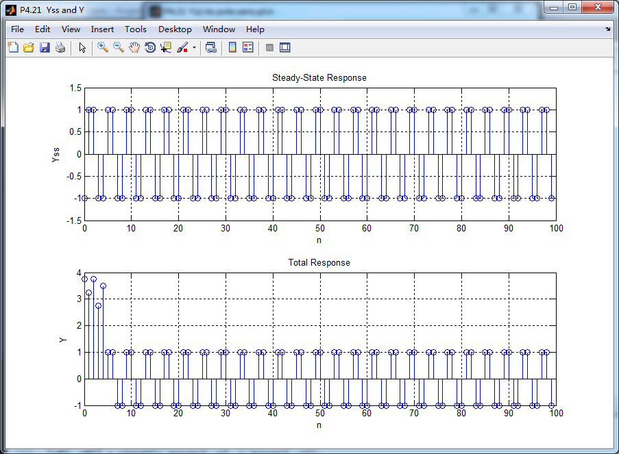
figure('NumberTitle', 'off', 'Name', 'P4.21  Yss and Y ');
set(gcf,'Color','white'); 
subplot(2,1,1); stem(n, y_answer5); grid on;  %axis([0,1,0,1.5]); 
title('Steady-State Response');
xlabel('n'); ylabel('Yss'); 
subplot(2,1,2); stem(n, y_check); grid on; % axis([-1,1,-1,1]);
title('Total Response');
xlabel('n'); ylabel('Y');

　　运行结果：

        系统函数H(z)的系数：

        系统的DTFT，注意当ω=π/2和π时的振幅谱、相位谱的值。

        当有输入时，输出的Y(z)进行部分分式展开，留数及对应的极点如下：

        单位圆上z=-1处，极点和零点相互抵消，稳态响应只和正负j有关。