

《DSP using MATLAB》Problem 3.20
代码:
%% ------------------------------------------------------------------------
%% Output Info about this m-file
fprintf('\n***********************************************************\n');
fprintf(' <DSP using MATLAB> Problem 3.20 \n\n');
banner();
%% ------------------------------------------------------------------------
%% -------------------------------------------------------------------
%% xa(t)=10cos(10000πt) through A/D
%% -------------------------------------------------------------------
Fs = 8000; % sample/sec
Ts = 1/Fs; % sample interval, 0.125ms=0.000125s
n1_start = -80; n1_end = 80;
n1 = [n1_start:1:n1_end];
nTs = n1 * Ts; % [-10,10]ms [-0.01,0.01]s
x1 = 10*cos(10000*pi*nTs); % Digital signal
M = 500;
[X1, w] = dtft1(x1, n1, M);
magX1 = abs(X1); angX1 = angle(X1); realX1 = real(X1); imagX1 = imag(X1);
%% --------------------------------------------------------------------
%% START X(w)'s mag ang real imag
%% --------------------------------------------------------------------
figure('NumberTitle', 'off', 'Name', 'Problem 3.20 X1');
set(gcf,'Color','white');
subplot(2,1,1); plot(w/pi,magX1); grid on; %axis([-1,1,0,1.05]);
title('Magnitude Response');
xlabel('frequency in \pi units'); ylabel('Magnitude |H|');
subplot(2,1,2); plot(w/pi, angX1/pi); grid on; %axis([-1,1,-1.05,1.05]);
title('Phase Response');
xlabel('frequency in \pi units'); ylabel('Radians/\pi');
figure('NumberTitle', 'off', 'Name', 'Problem 3.20 X1');
set(gcf,'Color','white');
subplot(2,1,1); plot(w/pi, realX1); grid on;
title('Real Part');
xlabel('frequency in \pi units'); ylabel('Real');
subplot(2,1,2); plot(w/pi, imagX1); grid on;
title('Imaginary Part');
xlabel('frequency in \pi units'); ylabel('Imaginary');
%% -------------------------------------------------------------------
%% END X's mag ang real imag
%% -------------------------------------------------------------------
%% --------------------------------------------------------
%% h(n) = (-0.9)^n[u(n)]
%% --------------------------------------------------------
n2 = n1;
h = (-0.9) .^ (n2) .* stepseq(0, n1_start, n1_end);
figure('NumberTitle', 'off', 'Name', 'Problem 3.20 h(n)');
set(gcf,'Color','white');
%subplot(2,1,1);
stem(n2, h); grid on; %axis([-1,1,0,1.05]);
title('Impulse Response: (-0.9)^n[u(n)]');
xlabel('n'); ylabel('h');
[H, w] = dtft1(h, n2, M);
magH = abs(H); angH = angle(H); realH = real(H); imagH = imag(H);
%% --------------------------------------------------------------------
%% START H(w)'s mag ang real imag
%% --------------------------------------------------------------------
figure('NumberTitle', 'off', 'Name', 'Problem 3.20 H');
set(gcf,'Color','white');
subplot(2,1,1); plot(w/pi,magH); grid on; %axis([-1,1,0,1.05]);
title('Magnitude Response');
xlabel('frequency in \pi units'); ylabel('Magnitude |H|');
subplot(2,1,2); plot(w/pi, angH/pi); grid on; %axis([-1,1,-1.05,1.05]);
title('Phase Response');
xlabel('frequency in \pi units'); ylabel('Radians/\pi');
figure('NumberTitle', 'off', 'Name', 'Problem 3.20 H');
set(gcf,'Color','white');
subplot(2,1,1); plot(w/pi, realH); grid on;
title('Real Part');
xlabel('frequency in \pi units'); ylabel('Real');
subplot(2,1,2); plot(w/pi, imagH); grid on;
title('Imaginary Part');
xlabel('frequency in \pi units'); ylabel('Imaginary');
%% -------------------------------------------------------------------
%% END X's mag ang real imag
%% -------------------------------------------------------------------
%% ----------------------------------------------
%% y(n)=x(n)*h(n)
%% ----------------------------------------------
[y, ny] = conv_m(x1, n1, h, n1);
figure('NumberTitle', 'off', 'Name', 'Problem 3.20 y(n)');
set(gcf,'Color','white');
%subplot(2,1,1);
stem(ny, y); grid on; %axis([-1,1,0,1.05]);
title('x(n)*h(n)');
xlabel('n'); ylabel('y');
[Y, w] = dtft1(y, ny, M);
magY = abs(Y); angY = angle(Y); realY = real(Y); imagY = imag(Y);
%% --------------------------------------------------------------------
%% START Y(w)'s mag ang real imag
%% --------------------------------------------------------------------
figure('NumberTitle', 'off', 'Name', 'Problem 3.20 Y');
set(gcf,'Color','white');
subplot(2,1,1); plot(w/pi,magY); grid on; %axis([-1,1,0,1.05]);
title('Magnitude Response');
xlabel('frequency in \pi units'); ylabel('Magnitude |H|');
subplot(2,1,2); plot(w/pi, angY/pi); grid on; %axis([-1,1,-1.05,1.05]);
title('Phase Response');
xlabel('frequency in \pi units'); ylabel('Radians/\pi');
figure('NumberTitle', 'off', 'Name', 'Problem 3.20 Y');
set(gcf,'Color','white');
subplot(2,1,1); plot(w/pi, realY); grid on;
title('Real Part');
xlabel('frequency in \pi units'); ylabel('Real');
subplot(2,1,2); plot(w/pi, imagY); grid on;
title('Imaginary Part');
xlabel('frequency in \pi units'); ylabel('Imaginary');
%% -------------------------------------------------------------------
%% END X's mag ang real imag
%% -------------------------------------------------------------------
%% ----------------------------------------------------------
%% xa(t) reconstruction from x1(n)
%% ----------------------------------------------------------
Dt = 0.00005; t = -0.01:Dt:0.01;
xa = x1 * sinc(Fs*(ones(length(n1),1)*t - nTs'*ones(1,length(t)))) ;
figure('NumberTitle', 'off', 'Name', 'Problem 3.20 Reconstructed From x1(n)');
set(gcf,'Color','white');
%subplot(2,1,1);
stairs(nTs*1000,x1); grid on; %axis([0,1,0,1.5]); % Zero-Order-Hold
title('Reconstructed Signal from x1(n) using zero-order-hold');
xlabel('t in msec.'); ylabel('xa(t)'); hold on;
stem(nTs*1000, x1); gtext('ZOH'); hold off;
figure('NumberTitle', 'off', 'Name', 'Problem 3.20 Reconstructed From x1(n)');
set(gcf,'Color','white');
%subplot(2,1,2);
plot(nTs*1000,x1); grid on; %axis([0,1,0,1.5]); % first-Order-Hold
title('Reconstructed Signal from x1(n) using first-Order-Hold');
xlabel('t in msec.'); ylabel('xa(t)'); hold on;
stem(nTs*1000,x1); gtext('FOH'); hold off;
xa = spline(nTs, x1, t);
figure('NumberTitle', 'off', 'Name', sprintf('Problem 3.20 Ts = %.6fs', Ts));
set(gcf,'Color','white');
%subplot(2,1,1);
plot(1000*t, xa);
xlabel('t in ms units'); ylabel('x');
title(sprintf('Reconstructed Signal from x1(n) using spline function')); grid on; hold on;
stem(1000*nTs, x1); gtext('spline');
%% ----------------------------------------------------------------
%% y(n) through D/A, reconstruction
%% ----------------------------------------------------------------
Dt = 0.00005; t = -0.02:Dt:0.02;
ya = y * sinc(Fs*(ones(length(ny),1)*t - (ny*Ts)'*ones(1,length(t)))) ;
figure('NumberTitle', 'off', 'Name', 'Problem 3.20 Reconstructed From y(n)');
set(gcf,'Color','white');
%subplot(2,1,1);
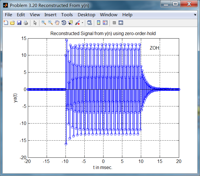
stairs(ny*Ts*1000,y); grid on; %axis([0,1,0,1.5]); % Zero-Order-Hold
title('Reconstructed Signal from y(n) using zero-order-hold');
xlabel('t in msec.'); ylabel('ya(t)'); hold on;
stem(ny*Ts*1000, y); gtext('ZOH'); hold off;
figure('NumberTitle', 'off', 'Name', 'Problem 3.20 Reconstructed From y(n)');
set(gcf,'Color','white');
%subplot(2,1,2);
plot(ny*Ts*1000,y); grid on; %axis([0,1,0,1.5]); % first-Order-Hold
title('Reconstructed Signal from y(n) using first-Order-Hold');
xlabel('t in msec.'); ylabel('ya(t)'); hold on;
stem(ny*Ts*1000,y); gtext('FOH'); hold off;
ya = spline(ny*Ts, y, t);
figure('NumberTitle', 'off', 'Name', sprintf('Problem 3.20 Ts = %.6fs', Ts));
set(gcf,'Color','white');
%subplot(2,1,1);
plot(1000*t, ya);
xlabel('t in ms units'); ylabel('y');
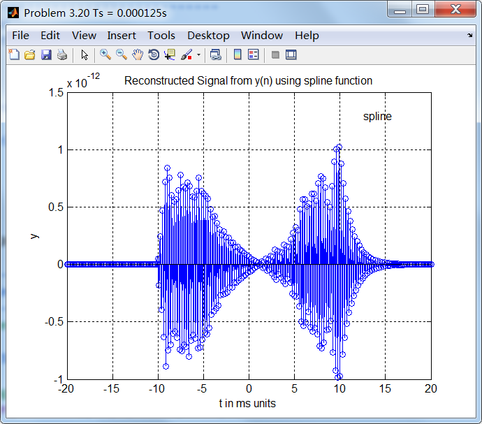
title(sprintf('Reconstructed Signal from y(n) using spline function')); grid on; hold on;
stem(1000*ny*Ts, y); gtext('spline');
运行结果:
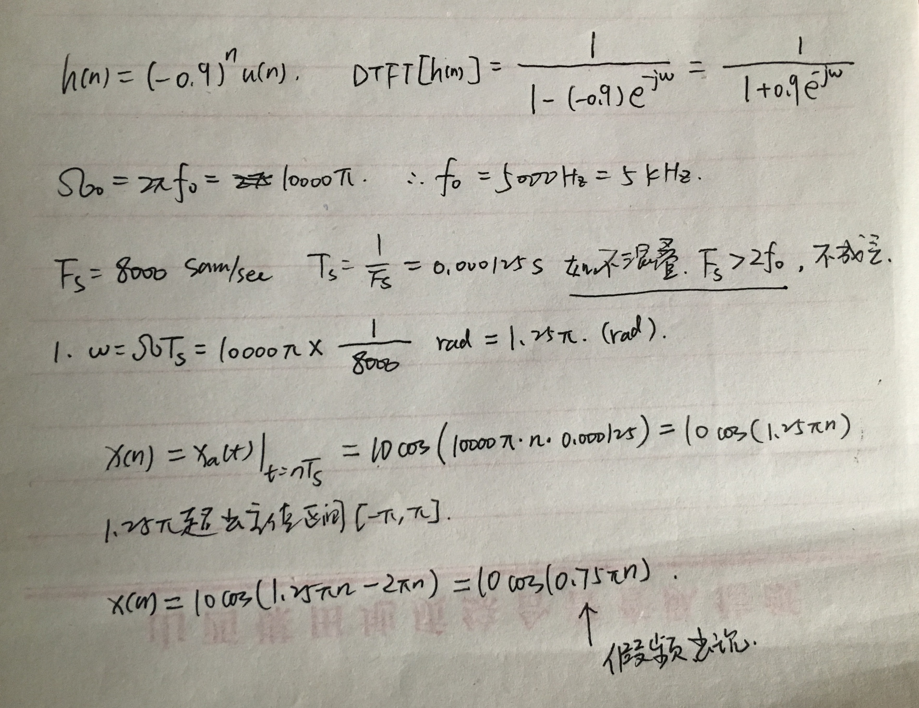
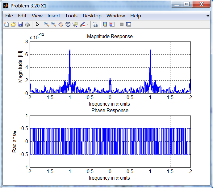
2、模拟信号经过Fs=8000sample/sec采样后,得采样信号的谱,如下图,0.75π处为假频。
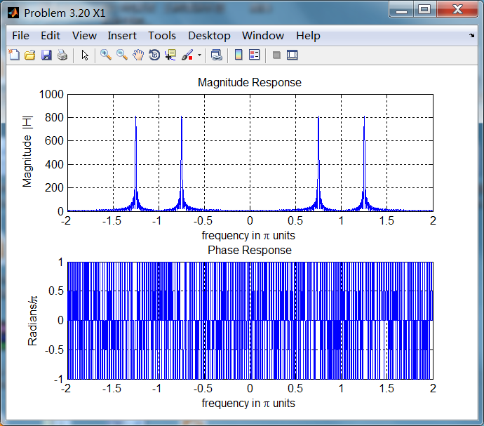
脉冲响应序列如下:
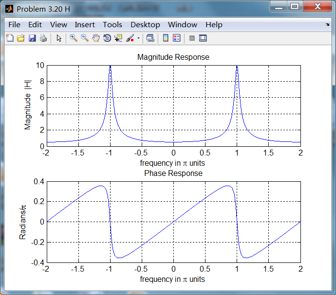
系统的频率响应,即脉冲响应序列的DTFT:
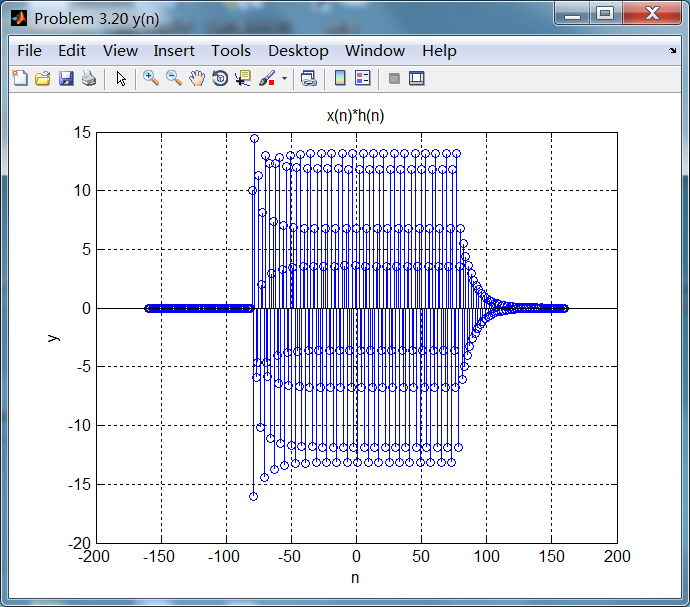
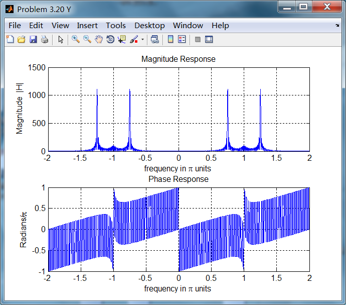
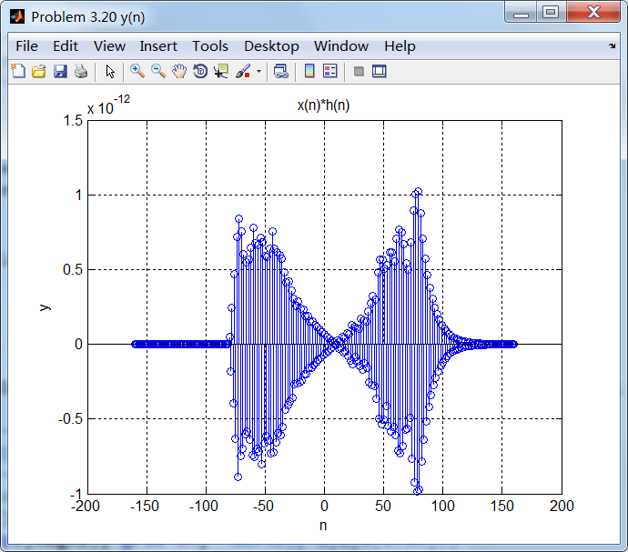
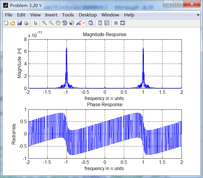
输出信号及其DTFT:
3、第3小题中的模拟信号经Fs=8000采样后,数字角频率为π,
采样后信号的谱:
采样后信号经过滤波器,输出信号的谱,
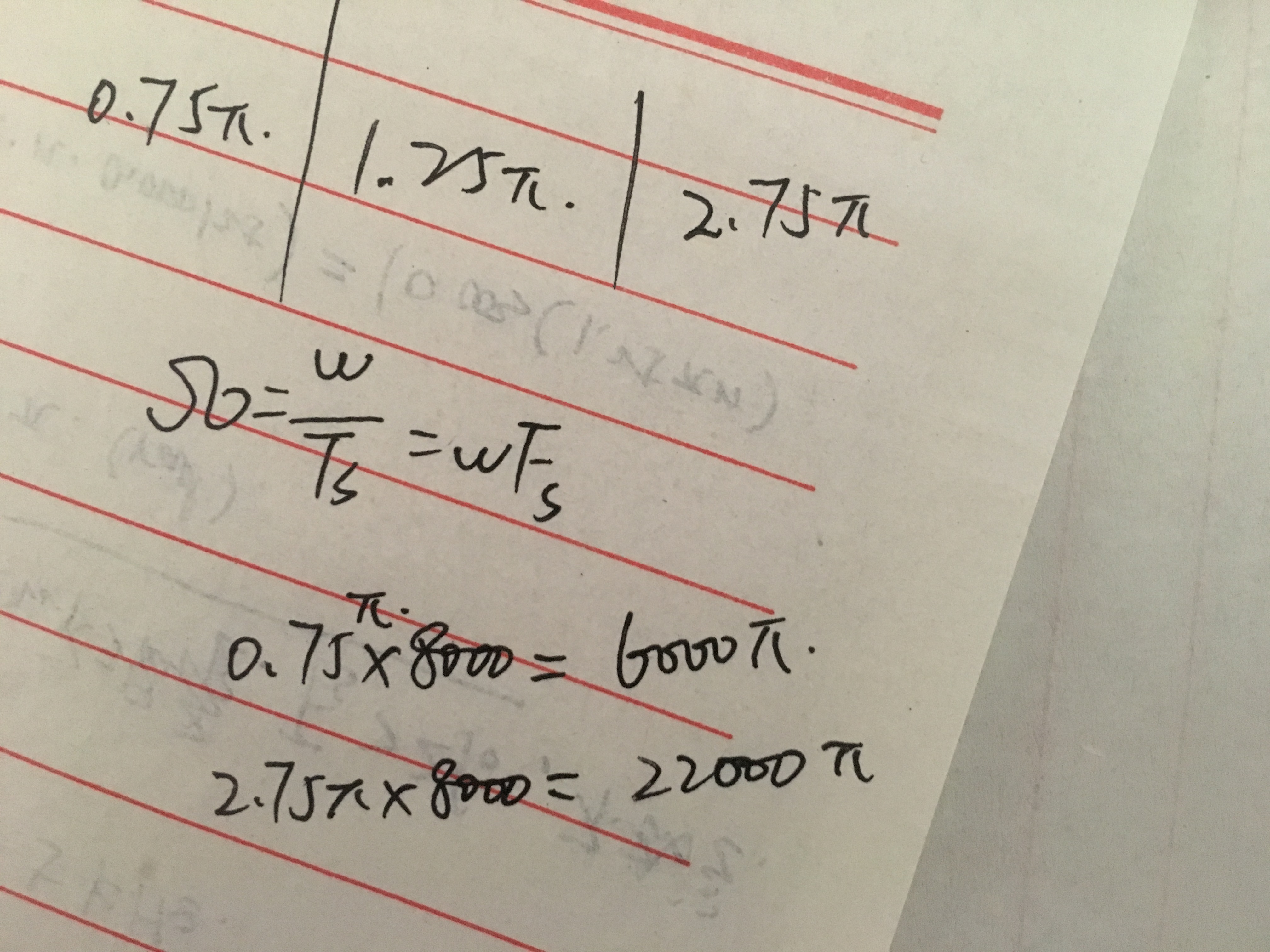
4、找到另外两个不同的模拟角频率的模拟信号,使得采样后和第1小题模拟信号采样后稳态输出相同。
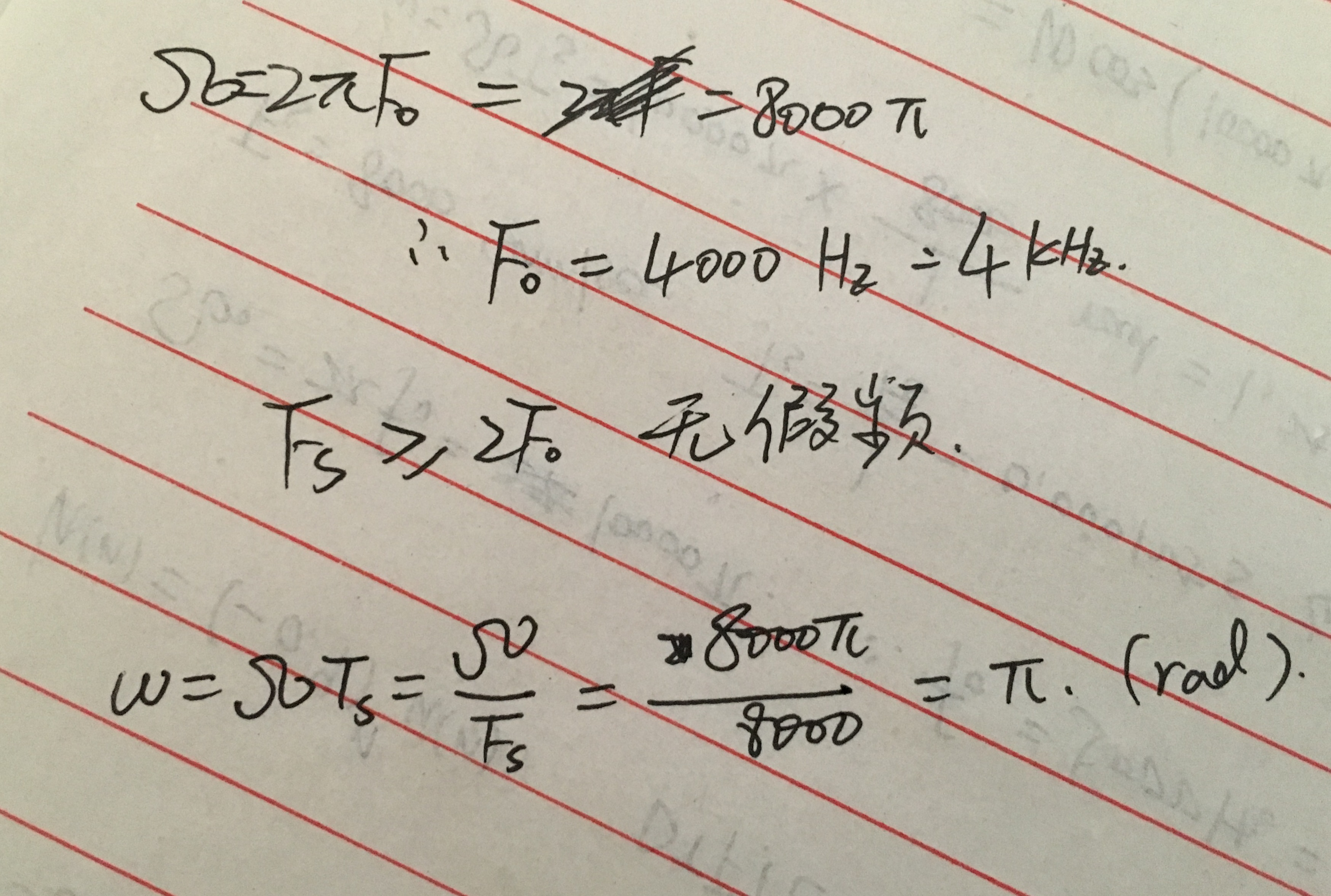
想求的数字角频率和第1题的数字角频率0.75π+2π,对应的模拟频率如下计算:
5、根据抽样定理,采用截止频率F0=4kHz,低通滤波器。

牢记:
1、如果你决定做某事,那就动手去做;不要受任何人、任何事的干扰。2、这个世界并不完美,但依然值得我们去为之奋斗。

 浙公网安备 33010602011771号