

《DSP using MATLAB》Problem 3.10(scilab脚本)
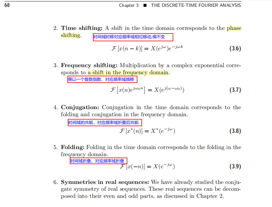
这里只做第4小题,使用到DTFT的频移性质,即将原始序列的谱直接频移,见下图第3点,
注:*****本文不对的地方请大家多批评指正*****。
一、上代码


  1 // Book Author:Vinay K Ingle, John G Proakis
  2 //
  3 // Problem 3.10
  4 // script by: KY
  5 //
  6 clear, clc, clf();
  7
  8 mode(2);
  9 funcprot(0);
 10 load('../fun/lib');
 11
 12 // -----------------------------------------------------------------------------
 13 //                START        Output Info about this sce-file
 14 mprintf('\n***********************************************************\n');
 15 [ban1,ban2] = fun_banner();
 16 mprintf("\n     <DSP using MATLAB> 3rd edition, Problem 3.10.4         \n");
 17 mprintf(" ----------------------------------------------------------\n\n");
 18
 19 // ----------------END----------------------------------------------------------
 20
 21 //% ------------------------------------------------------------------
 22 //%                Triangular Window sequence, and its DTFT
 23 //% ------------------------------------------------------------------
 24 //M = 10;
 25 //M = 15;
 26 M = 25;
 27 //M = 100;
 28
 29 n1_start = 0; n1_end = M;
 30 n1 = [n1_start : n1_end - 1];
 31
 32 x1 = (1 - abs(M-1-2*n1)/(M-1)) .* ones(1, length(n1));
 33
 34 // -----------------------------------------------------------------------------
 35 // --------------------START  f0 figure-----------------------------------------
 36 f0=scf(0);                    //creates figure with id==0 and make it the current one
 37   f0.figure_size=[1000,700];               // adjust window size
 38   f0.background=8;                         // add background color 8-white
 39   f0.figure_name=msprintf("Fig0 Problem 3.10.4 x1(n) Triangular, M = %d",M); // name window
 40
 41      plot(n1,x1,'bo');
 42      plot(n1,x1,'b.');
 43   plot2d3(n1,x1,2);                   // Create plot with blue line
 44 //title("$x1(n)\ sequence\ Rectangle, M = 100$",'fontname',7,'fontsize',4);
 45 title(msprintf('x1(n)=Tm(n) Triangular sequence , M = %d', M));
 46 xlabel('$n$','fontname',3); ylabel('x1','fontname',3,'fontsize',3);
 47 xgrid(5,0,7);                             // color, thickness, style
 48 a0=get("current_axes");                   // get the handle of the newly created axes
 49 //a0.data_bounds=[-4,6,-6,6];
 50 // -----------------------------------------------------------------------------
 51 // --------------------END  f0 -------------------------------------------------
 52
 53
 54 MM = 500;
 55 k = [-MM:MM];        // [-pi, pi]
 56 //k = [0:M];        // [0, pi]
 57 w = (%pi/MM) * k;
 58
 59 [X1] = fun_dtft(x1, n1, w);
 60
 61 magX1 = abs(X1); angX1 = fun_angle(X1); realX1 = real(X1); imagX1 = imag(X1);
 62
 63 //%% ---------------------------------------------------------------------------
 64 //%%                   START X(w)'s  mag ang real imag
 65 // --------------------START  f1 figure-----------------------------------------
 66 f1=scf(1);                    //creates figure with id==0 and make it the current one
 67   f1.figure_size=[1000,700];               // adjust window size
 68   f1.background=8;                         // add background color 8-white
 69   f1.figure_name=msprintf("Fig1 Problem 3.10.4 DTFT of Tm(n), M = %d",M); // name window
 70   subplot(2, 2, 1);
 71      plot(w/%pi,magX1);
 72 title("$Magnitude\ Response$",'fontname',7,'fontsize',4);
 73 xlabel('$frequency\ in\ \pi\ units$','fontname',3); ylabel('Magnitude |X|','fontname',3,'fontsize',3);
 74 xgrid(5,0,7);                             // color, thickness, style
 75 a0=get("current_axes");                   // get the handle of the newly created axes
 76 //a0.data_bounds=[-4,6,-6,6];
 77
 78  subplot(2, 2, 3);
 79      plot(w/%pi,angX1/%pi*exp(20));
 80 title("$Phase\ Response$",'fontname',7,'fontsize',4);
 81 xlabel('$frequency\ in\ \pi\ units$','fontname',3); ylabel('$Radians/\pi*exp(20)$','fontname',3,'fontsize',3);
 82 xgrid(5,1,7);                            // color, thickness, style
 83 a1=get("current_axes");                  // get the handle of the newly created axes
 84 //a1.data_bounds=[-4,6,-2,2];
 85
 86  subplot(2, 2, 2);
 87      plot(w/%pi,realX1);
 88 title("$Real\ Part$",'fontname',7,'fontsize',4);
 89 xlabel('$frequency\ in\ \pi\ units$','fontname',3); ylabel('Real','fontname',3,'fontsize',3);
 90 //xgrid();
 91 xgrid(5,1,7);                           // color, thickness, style
 92 a2=get("current_axes");                 // get the handle of the newly created axes
 93 //a2.data_bounds=[-4,6,-2,2];
 94
 95  subplot(2, 2, 4);
 96      plot(w/%pi,imagX1*exp(20));
 97 title("$Imaginary\ Part$",'fontname',7,'fontsize',4);
 98 xlabel('$frequency\ in\ \pi\ units$','fontname',3); ylabel('Imaginary*exp(20)','fontname',3,'fontsize',3);
 99 //xgrid();
100 xgrid(5,1,7);                          // color, thickness, style
101 a3=get("current_axes");                // get the handle of the newly created axes
102 //a2.data_bounds=[-4,6,-2,2];
103 // ----------------------------END f1-------------------------------------------
104 //%%                   END X(w)'s  mag ang real imag
105 //%% ---------------------------------------------------------------------------
106
107
108
109 //%% ---------------------------------------------------------------
110 //%%                  exp(jπn)  and its DTFT
111 //%% ---------------------------------------------------------------
112 n2 = n1;
113 x2 = exp(%i * %pi * n2);
114
115 // -----------------------------------------------------------------------------
116 // --------------------START  f2 figure-----------------------------------------
117 f2=scf(2);                    //creates figure with id==0 and make it the current one
118   f2.figure_size=[1000,700];               // adjust window size
119   f2.background=8;                         // add background color 8-white
120   f2.figure_name=msprintf("Fig2 Problem 3.10.4 x2(n)=exp(iπn), M = %d",M); // name window
121   subplot(2, 1, 1);
122      plot(n2,real(x2),'bo');
123      plot(n2,real(x2),'b.');
124   plot2d3(n2,real(x2),2);                   // Create plot with blue line
125 title(msprintf('Real Part of x2(n)=exp(iπn) sequence , M = %d', M));
126 xlabel('$n$','fontname',3); ylabel('x2','fontname',3,'fontsize',3);
127 xgrid(5,0,7);                             // color, thickness, style
128 a0=get("current_axes");                   // get the handle of the newly created axes
129 //a0.data_bounds=[-4,6,-6,6];
130
131  subplot(2, 1, 2);
132      plot(n2,imag(x2)*exp(20),'bo');
133      plot(n2,imag(x2)*exp(20),'b.');
134   plot2d3(n2,imag(x2)*exp(20),2);                   // Create plot with blue line
135 title(msprintf('Imaginary Part of x2(n)=exp(iπn)*exp(20) sequence , M = %d', M));
136 xlabel('$n$','fontname',3); ylabel('x2','fontname',3,'fontsize',3);
137 xgrid(5,0,7);                             // color, thickness, style
138 a1=get("current_axes");                   // get the handle of the newly created axes
139 //a1.data_bounds=[-4,6,-6,6];
140 // --------------------END  f2 -------------------------------------------------
141 // -----------------------------------------------------------------------------
142
143
144 MM = 500;
145 k = [-MM:MM];        // [-pi, pi]
146 //k = [0:M];        // [0, pi]
147 w = (%pi/MM) * k;
148
149 [X2] = fun_dtft(x2, n2, w);
150
151 magX2 = abs(X2); angX2 = fun_angle(X2); realX2 = real(X2); imagX2 = imag(X2);
152
153 //%% ---------------------------------------------------------------------------
154 //%%                   START X(w)'s  mag ang real imag
155 // --------------------START  f3 figure-----------------------------------------
156 f3=scf(3);                    //creates figure with id==0 and make it the current one
157   f3.figure_size=[1000,700];               // adjust window size
158   f3.background=8;                         // add background color 8-white
159   f3.figure_name=msprintf("Fig3 Problem 3.10.4 DTFT of x2(n)=exp(iπn), M = %d",M); // name window
160   subplot(2, 2, 1);
161      plot(w/%pi,magX2);
162 title("$Magnitude\ Response$",'fontname',7,'fontsize',4);
163 xlabel('$frequency\ in\ \pi\ units$','fontname',3); ylabel('Magnitude |X|','fontname',3,'fontsize',3);
164 xgrid(5,0,7);                             // color, thickness, style
165 a0=get("current_axes");                   // get the handle of the newly created axes
166 //a0.data_bounds=[-4,6,-6,6];
167
168  subplot(2, 2, 3);
169      plot(w/%pi,angX2/%pi*exp(20));
170 title("$Phase\ Response$",'fontname',7,'fontsize',4);
171 xlabel('$frequency\ in\ \pi\ units$','fontname',3); ylabel('$Radians/\pi*exp(20)$','fontname',3,'fontsize',3);
172 xgrid(5,1,7);                            // color, thickness, style
173 a1=get("current_axes");                  // get the handle of the newly created axes
174 //a1.data_bounds=[-4,6,-2,2];
175
176  subplot(2, 2, 2);
177      plot(w/%pi,realX2);
178 title("$Real\ Part$",'fontname',7,'fontsize',4);
179 xlabel('$frequency\ in\ \pi\ units$','fontname',3); ylabel('Real','fontname',3,'fontsize',3);
180 //xgrid();
181 xgrid(5,1,7);                           // color, thickness, style
182 a2=get("current_axes");                 // get the handle of the newly created axes
183 //a2.data_bounds=[-4,6,-2,2];
184
185  subplot(2, 2, 4);
186      plot(w/%pi,imagX2*exp(20));
187 title("$Imaginary\ Part$",'fontname',7,'fontsize',4);
188 xlabel('$frequency\ in\ \pi\ units$','fontname',3); ylabel('Imaginary*exp(20)','fontname',3,'fontsize',3);
189 //xgrid();
190 xgrid(5,1,7);                          // color, thickness, style
191 a3=get("current_axes");                // get the handle of the newly created axes
192 //a2.data_bounds=[-4,6,-2,2];
193 // ----------------------------END f3-------------------------------------------
194 //%%                   END X(w)'s  mag ang real imag
195 //%% ---------------------------------------------------------------------------
196
197
198 //%% -----------------------------------------------------------------
199 //%%                 Tm(n)*exp(jπn) and its DTFT
200 //%% -----------------------------------------------------------------
201 [x3, n3] = fun_sigmult(x1, n1, x2, n2);
202
203 // -----------------------------------------------------------------------------
204 // --------------------START  f4 figure-----------------------------------------
205 f4=scf(4);                    //creates figure with id==0 and make it the current one
206   f4.figure_size=[1000,700];               // adjust window size
207   f4.background=8;                         // add background color 8-white
208   f4.figure_name=msprintf("Fig4 Problem 3.10.4 x3(n)=Tm(n)exp(iπn), M = %d",M); // name window
209   subplot(2, 1, 1);
210      plot(n3,real(x3),'bo');
211      plot(n3,real(x3),'b.');
212   plot2d3(n3,real(x3),2);                   // Create plot with blue line
213 title(msprintf('Real Part of x3(n)=Tm(n)exp(iπn) sequence , M = %d', M));
214 xlabel('$n$','fontname',3); ylabel('x3','fontname',3,'fontsize',3);
215 xgrid(5,0,7);                             // color, thickness, style
216 a0=get("current_axes");                   // get the handle of the newly created axes
217 //a0.data_bounds=[-4,6,-6,6];
218
219  subplot(2, 1, 2);
220      plot(n3,imag(x3)*exp(20),'bo');
221      plot(n3,imag(x3)*exp(20),'b.');
222   plot2d3(n3,imag(x3)*exp(20),2);                   // Create plot with blue line
223 title(msprintf('Imaginary Part of x3(n)=Tm(n)exp(iπn)*exp(20) sequence , M = %d', M));
224 xlabel('$n$','fontname',3); ylabel('x3','fontname',3,'fontsize',3);
225 xgrid(5,0,7);                             // color, thickness, style
226 a1=get("current_axes");                   // get the handle of the newly created axes
227 //a1.data_bounds=[-4,6,-6,6];
228 // --------------------END  f4 -------------------------------------------------
229 // -----------------------------------------------------------------------------
230
231
232 MM = 500;
233 k = [-MM:MM];        // [-pi, pi]
234 //k = [0:M];        // [0, pi]
235 w = (%pi/MM) * k;
236
237 [X3] = fun_dtft(x3, n3, w);
238
239 magX3 = abs(X3); angX3 = fun_angle(X3); realX3 = real(X3); imagX3 = imag(X3);
240
241 //%% ---------------------------------------------------------------------------
242 //%%                   START X(w)'s  mag ang real imag
243 // --------------------START  f5 figure-----------------------------------------
244 f5=scf(5);                    //creates figure with id==0 and make it the current one
245   f5.figure_size=[1000,700];               // adjust window size
246   f5.background=8;                         // add background color 8-white
247   f5.figure_name=msprintf("Fig5 Problem 3.10.4 DTFT of x3(n)=Tm(n)exp(iπn), M = %d",M);  // name window
248   subplot(2, 2, 1);
249      plot(w/%pi,magX3);
250 title("$Magnitude\ Response$",'fontname',7,'fontsize',4);
251 xlabel('$frequency\ in\ \pi\ units$','fontname',3); ylabel('Magnitude |X|','fontname',3,'fontsize',3);
252 xgrid(5,0,7);                             // color, thickness, style
253 a0=get("current_axes");                   // get the handle of the newly created axes
254 //a0.data_bounds=[-4,6,-6,6];
255
256  subplot(2, 2, 3);
257      plot(w/%pi,angX3/%pi*exp(20));
258 title("$Phase\ Response$",'fontname',7,'fontsize',4);
259 xlabel('$frequency\ in\ \pi\ units$','fontname',3); ylabel('$Radians/\pi*exp(20)$','fontname',3,'fontsize',3);
260 xgrid(5,1,7);                            // color, thickness, style
261 a1=get("current_axes");                  // get the handle of the newly created axes
262 //a1.data_bounds=[-4,6,-2,2];
263
264  subplot(2, 2, 2);
265      plot(w/%pi,realX3);
266 title("$Real\ Part$",'fontname',7,'fontsize',4);
267 xlabel('$frequency\ in\ \pi\ units$','fontname',3); ylabel('Real','fontname',3,'fontsize',3);
268 //xgrid();
269 xgrid(5,1,7);                           // color, thickness, style
270 a2=get("current_axes");                 // get the handle of the newly created axes
271 //a2.data_bounds=[-4,6,-2,2];
272
273  subplot(2, 2, 4);
274      plot(w/%pi,imagX3*exp(20));
275 title("$Imaginary\ Part$",'fontname',7,'fontsize',4);
276 xlabel('$frequency\ in\ \pi\ units$','fontname',3); ylabel('Imaginary*exp(20)','fontname',3,'fontsize',3);
277 //xgrid();
278 xgrid(5,1,7);                          // color, thickness, style
279 a3=get("current_axes");                // get the handle of the newly created axes
280 //a2.data_bounds=[-4,6,-2,2];
281 // ----------------------------END f5-------------------------------------------
282 //%%                   END X(w)'s  mag ang real imag
283 //%% ---------------------------------------------------------------------------
284
285
286 //%% ------------------------------------------------------
287 //%%           Properties of DTFT
288 //%% ------------------------------------------------------
289
290 [X3_check, n3_check] = fun_sigshift(X1, w/%pi*500, 500);
291
292 //error = clean(max(abs(X3-X3_check)));              // Difference
293 //mprintf("\n abs(X3-X3_check) = %.2f\n", error);
294
295
296 magX3C = abs(X3_check); angX3C = fun_angle(X3_check); realX3C = real(X3_check); imagX3C = imag(X3_check);
297
298 //%% ---------------------------------------------------------------------------
299 //%%                   START X(w)'s  mag ang real imag
300 // --------------------START  f6 figure-----------------------------------------
301 f6=scf(6);                    //creates figure with id==0 and make it the current one
302   f6.figure_size=[1000,700];               // adjust window size
303   f6.background=8;                         // add background color 8-white
304   f6.figure_name=msprintf("Fig6 Problem 3.10.4 X3C=X1(w-π), M = %d",M);  // name window
305   subplot(2, 2, 1);
306 //     plot(w/%pi,magX3C);
307      plot(n3_check/MM,magX3C);
308 title("$Magnitude\ Response$",'fontname',7,'fontsize',4);
309 xlabel('$frequency\ in\ \pi\ units$','fontname',3); ylabel('Magnitude |X|','fontname',3,'fontsize',3);
310 xgrid(5,0,7);                             // color, thickness, style
311 a0=get("current_axes");                   // get the handle of the newly created axes
312 //a0.data_bounds=[-4,6,-6,6];
313
314  subplot(2, 2, 3);
315 //     plot(w/%pi,angX3C/%pi*exp(20));
316     plot(n3_check/MM,angX3C/%pi*exp(20));
317 title("$Phase\ Response$",'fontname',7,'fontsize',4);
318 xlabel('$frequency\ in\ \pi\ units$','fontname',3); ylabel('$Radians/\pi*exp(20)$','fontname',3,'fontsize',3);
319 xgrid(5,1,7);                            // color, thickness, style
320 a1=get("current_axes");                  // get the handle of the newly created axes
321 //a1.data_bounds=[-4,6,-2,2];
322
323  subplot(2, 2, 2);
324 //     plot(w/%pi,realX3C);
325       plot(n3_check/MM,realX3C);
326 title("$Real\ Part$",'fontname',7,'fontsize',4);
327 xlabel('$frequency\ in\ \pi\ units$','fontname',3); ylabel('Real','fontname',3,'fontsize',3);
328 //xgrid();
329 xgrid(5,1,7);                           // color, thickness, style
330 a2=get("current_axes");                 // get the handle of the newly created axes
331 //a2.data_bounds=[-4,6,-2,2];
332
333  subplot(2, 2, 4);
334 //     plot(w/%pi,imagX3C*exp(20));
335      plot(n3_check/MM,imagX3C*exp(20));
336 title("$Imaginary\ Part$",'fontname',7,'fontsize',4);
337 xlabel('$frequency\ in\ \pi\ units$','fontname',3); ylabel('Imaginary*exp(20)','fontname',3,'fontsize',3);
338 //xgrid();
339 xgrid(5,1,7);                          // color, thickness, style
340 a3=get("current_axes");                // get the handle of the newly created axes
341 //a2.data_bounds=[-4,6,-2,2];
342 // ----------------------------END f6-------------------------------------------
343 //%%                   END X(w)'s  mag ang real imag
344 //%% ---------------------------------------------------------------------------
二、运行结果
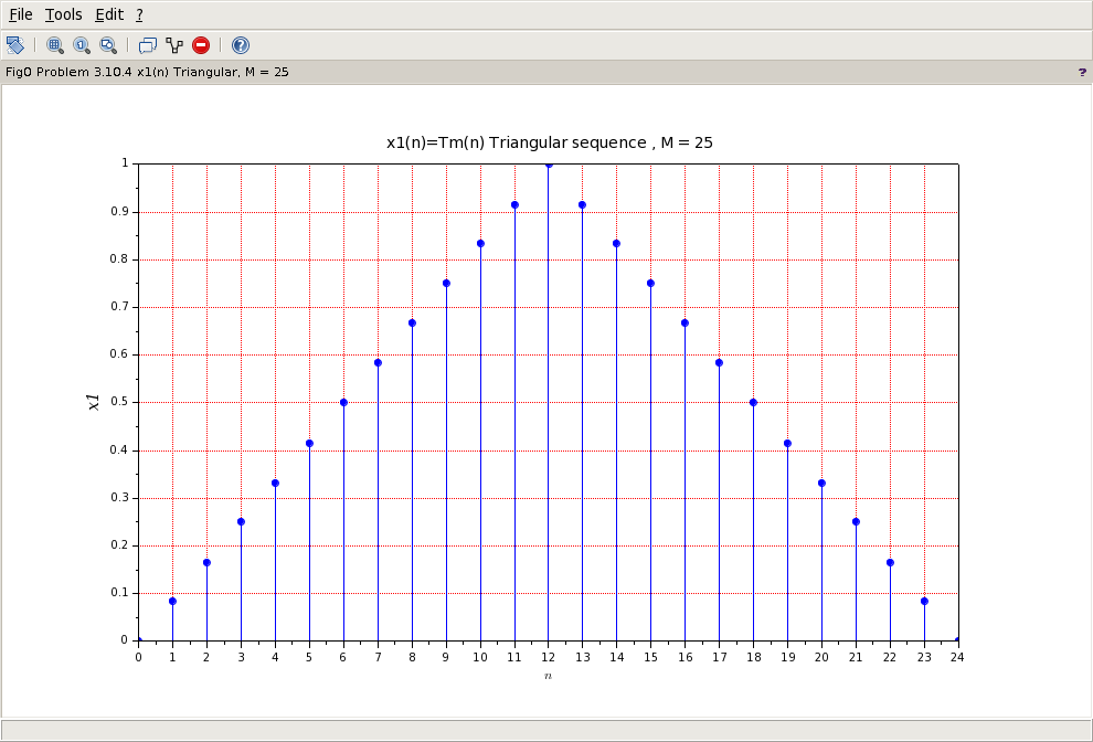
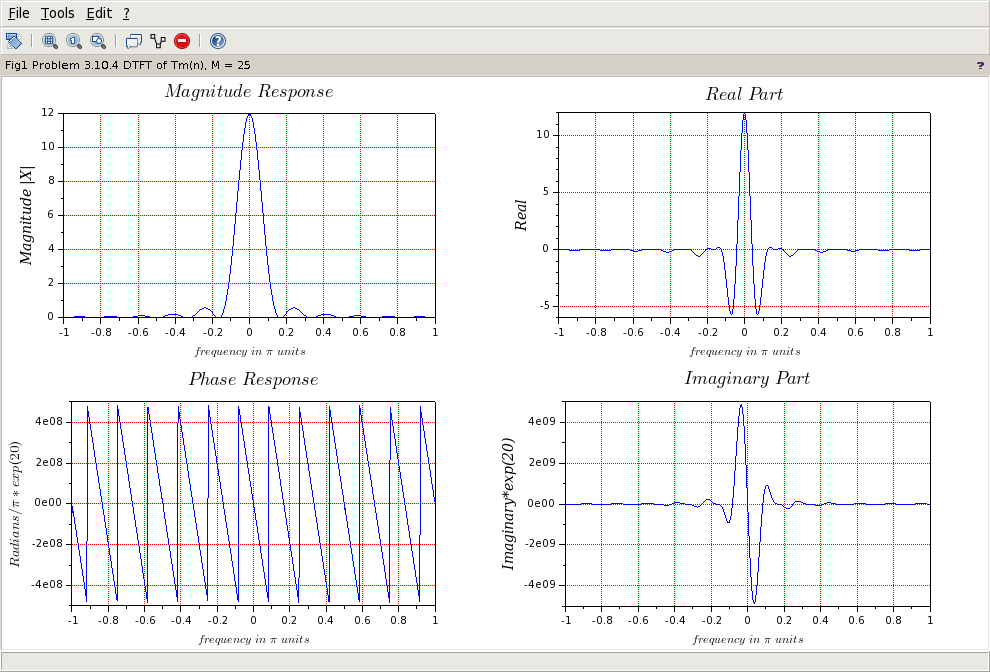
1、原始三角序列和谱,长度为M=25
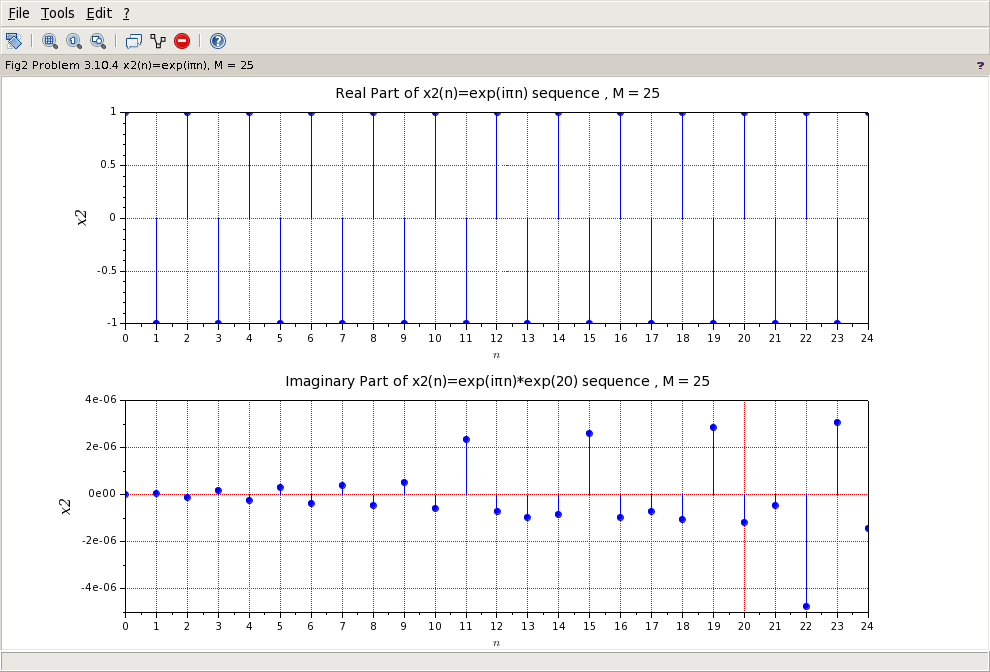
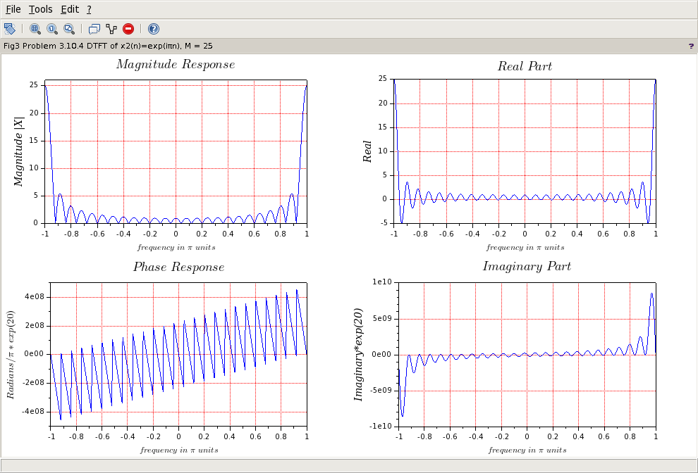
2、指数序列exp(jπn),和谱。虚部是sin(πn),理论值是0,估计是计算机内部数值表示的缘故,scilab用科学计数法表示,都是e的-16次幂,可以认为是0了。
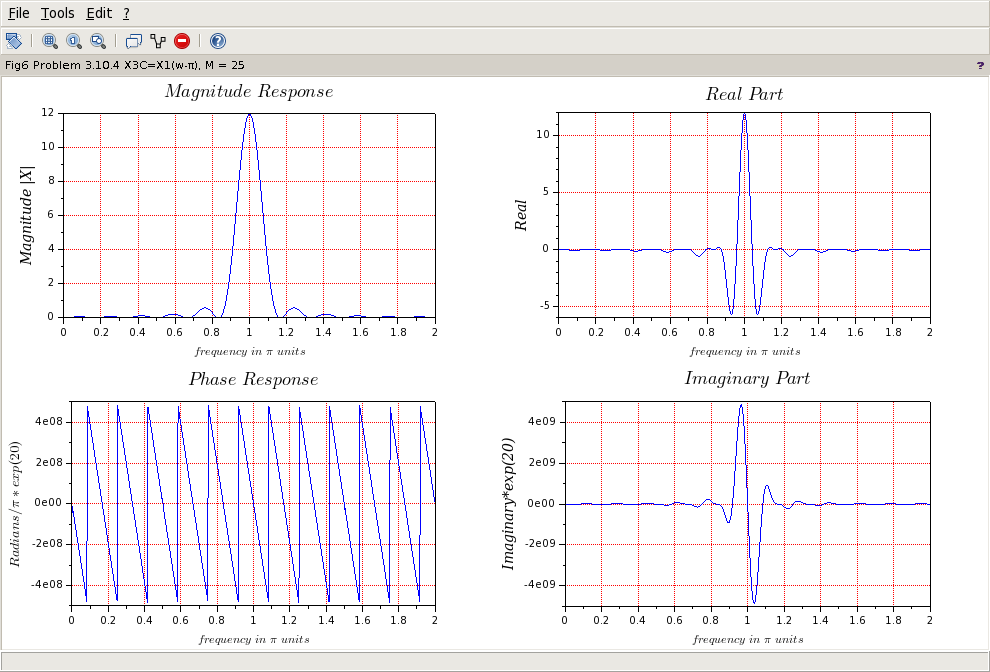
3、原始三角序列和指数序列相乘,并计算谱,

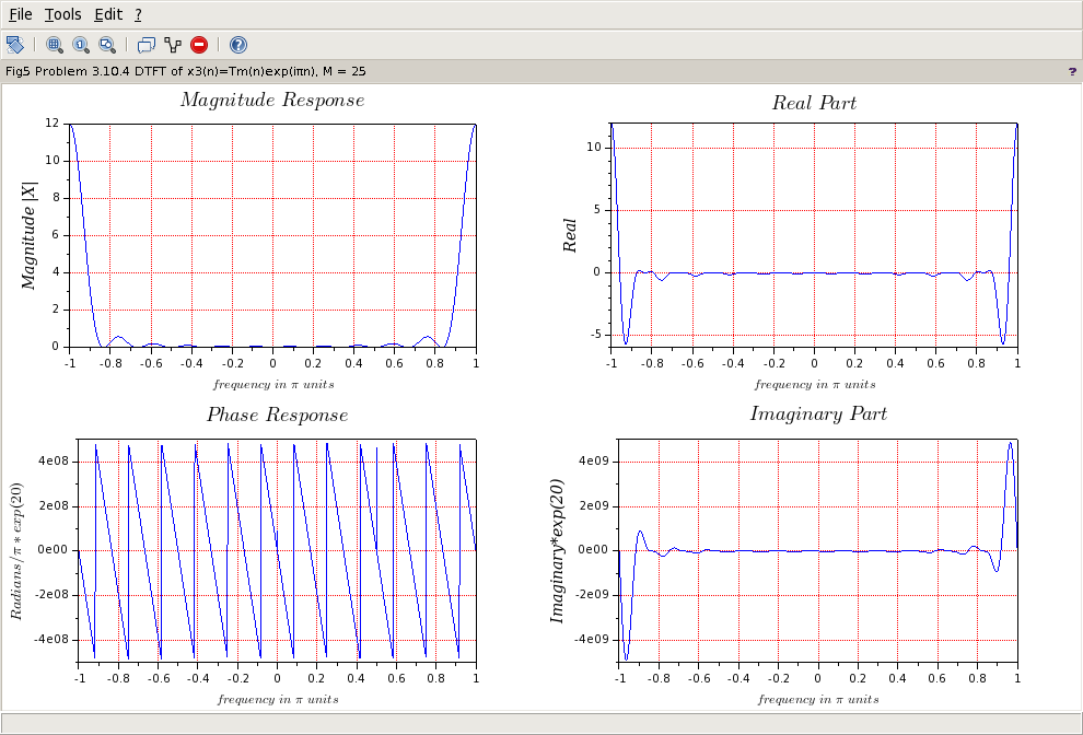
4、上图可以看成是将原始三角序列的谱直接平移π个单位得到的,注意DTFT的周期性(2π为基本周期)。
牢记:
1、如果你决定做某事,那就动手去做;不要受任何人、任何事的干扰。2、这个世界并不完美,但依然值得我们去为之奋斗。

 浙公网安备 33010602011771号