

《DSP using MATLAB》Problem 8.40
代码:
function [wpLP, wsLP, alpha] = bs2lpfre(wpbs, wsbs)
% Band-edge frequency conversion from bandstop to lowpass digital filter
% -------------------------------------------------------------------------
% [wpLP, wsLP, alpha] = bs2lpfre(wpbs, wsbs)
%   wpLP = passband edge for the lowpass digital prototype
%   wsLP = stopband edge for the lowpass digital prototype
%  alpha = lowpass to bandstop transformation parameter
%   wpbs = passband edge frequency array [wp_lower, wp_upper] for the bandstop
%   wsbs = stopband edge frequency array [ws_lower, ws_upper] for the bandstop
%
%

% Determine the digital lowpass cutoff frequencies:
wpLP = 0.2*pi;
     K = tan((wpbs(2)-wpbs(1))/2)*tan(wpLP/2);
  beta = cos((wpbs(2)+wpbs(1))/2)/cos((wpbs(2)-wpbs(1))/2);
alpha1 = -2*beta*K/(K+1);
alpha2 = (1-K)/(K+1);

alpha = [alpha1, alpha2];

wsLP = -angle((exp(-2*j*wsbs(1))+alpha1*exp(-j*wsbs(1))+alpha2)/(alpha2*exp(-2*j*wsbs(1))+alpha1*exp(-j*wsbs(1))+1))
wsLP = angle((exp(-2*j*wsbs(2))+alpha1*exp(-j*wsbs(2))+alpha2)/(alpha2*exp(-2*j*wsbs(2))+alpha1*exp(-j*wsbs(2))+1))
function [b, a] = cheb1bsf(wpbs, wsbs, Rp, As)
% IIR bandstop Filter Design using Chebyshev-1 Prototype
% -----------------------------------------------------------------------
% [b, a] = cheb1bsf(wp, ws, Rp, As);
%      b = numerator polynomial coefficients of bandstop filter, Direct form
%      a = denominator polynomial coefficients of bandstop filter, Direct form
%     wp = Passband edge frequency array [wp_lower, wp_upper] in radians;
%     ws = Stopband edge frequency array [ws_lower, ws_upper] in radians;
%     Rp = Passband ripple in +dB; Rp > 0
%     As = Stopband attenuation in +dB; As > 0
%
%
% Determine the digital lowpass cutoff frequencies:
wpLP = 0.2*pi;
     K = tan((wpbs(2)-wpbs(1))/2)*tan(wpLP/2);
  beta = cos((wpbs(2)+wpbs(1))/2)/cos((wpbs(2)-wpbs(1))/2);
alpha1 = -2*beta*K/(K+1);
alpha2 = (1-K)/(K+1);

alpha = [alpha1, alpha2];

wsLP = -angle((exp(-2*j*wsbs(1))+alpha1*exp(-j*wsbs(1))+alpha2)/(alpha2*exp(-2*j*wsbs(1))+alpha1*exp(-j*wsbs(1))+1))
wsLP = angle((exp(-2*j*wsbs(2))+alpha1*exp(-j*wsbs(2))+alpha2)/(alpha2*exp(-2*j*wsbs(2))+alpha1*exp(-j*wsbs(2))+1))

% Compute Analog Lowpass Prototype Specifications: Inverse Mapping for frequencies
T = 1; Fs = 1/T;                    % set T = 1
OmegaP = (2/T)*tan(wpLP/2);         % Prewarp(Cutoff) prototype passband freq
OmegaS = (2/T)*tan(wsLP/2);         % Prewarp(cutoff) prototype stopband freq

% Design Analog Chebyshev-1 Prototype Lowpass Filter:
[cs, ds] = afd_chb1(OmegaP, OmegaS, Rp, As);

% Bilinear transformation to obtain digital lowpass:
[blp, alp] = bilinear(cs, ds, Fs);

% Transform digital lowpass into bandstop filter
Nz = [alpha2, alpha1, 1]; Dz = [1, alpha1, alpha2];
[b, a] = zmapping(blp, alp, Nz, Dz);
%% ------------------------------------------------------------------------
%% Output Info about this m-file
fprintf('\n***********************************************************\n');
fprintf(' <DSP using MATLAB> Problem 8.40.2 \n\n');
banner();
%% ------------------------------------------------------------------------
% Digital Filter Specifications: Chebyshev-1 bandstop
wsbs = [0.35*pi 0.65*pi]; % digital stopband freq in rad
wpbs = [0.25*pi 0.75*pi]; % digital passband freq in rad
delta1 = 0.05; % passband tolerance, absolute specs
delta2 = 0.01; % stopband tolerance, absolute specs
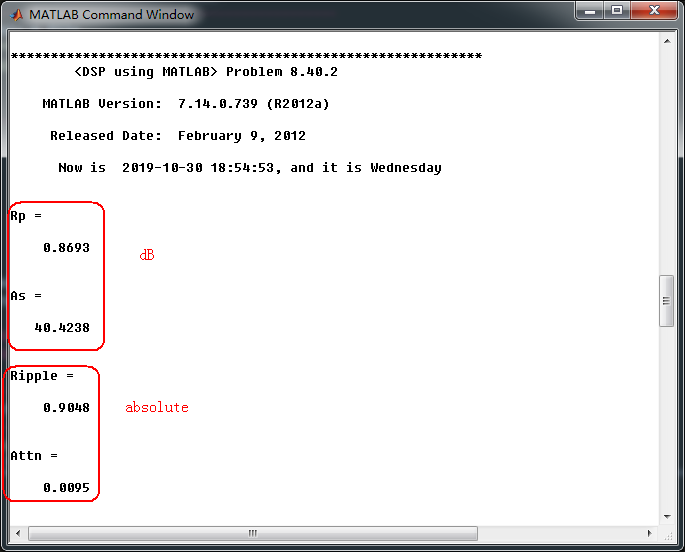
Rp = -20 * log10( (1-delta1)/(1+delta1)) % passband ripple in dB
As = -20 * log10( delta2 / (1+delta1)) % stopband attenuation in dB
Ripple = 10 ^ (-Rp/20) % passband ripple in absolute
Attn = 10 ^ (-As/20) % stopband attenuation in absolute
% --------------------------------------------------------
% method 1: cheb1bsf function
% --------------------------------------------------------
fprintf('\n*******Digital bandstop, Coefficients of DIRECT-form***********\n');
[bbs, abs] = cheb1bsf(wpbs, wsbs, Rp, As)
[C, B, A] = dir2cas(bbs, abs)
% Calculation of Frequency Response:
[dbbs, magbs, phabs, grdbs, wwbs] = freqz_m(bbs, abs);
% ---------------------------------------------------------------
% find Actual Passband Ripple and Min Stopband attenuation
% ---------------------------------------------------------------
delta_w = 2*pi/1000;
Rp_bs = -(min(dbbs( 1:1:ceil(wpbs(1)/delta_w+1) ))); % Actual Passband Ripple
fprintf('\nActual Passband Ripple is %.4f dB.\n', Rp_bs);
As_bs = -round(max(dbbs(ceil(wsbs(1)/delta_w)+1:1:ceil(wsbs(2)/delta_w)+1))); % Min Stopband attenuation
fprintf('\nMin Stopband attenuation is %.4f dB.\n\n', As_bs);
%% -----------------------------------------------------------------
%% Plot
%% -----------------------------------------------------------------
figure('NumberTitle', 'off', 'Name', 'Problem 8.40.2 Chebyshev-1 bs by cheb1bsf function')
set(gcf,'Color','white');
M = 1; % Omega max
subplot(2,2,1); plot(wwbs/pi, magbs); axis([0, M, 0, 1.2]); grid on;
xlabel('Digital frequency in \pi units'); ylabel('|H|'); title('Magnitude Response');
set(gca, 'XTickMode', 'manual', 'XTick', [0, 0.25, 0.35, 0.65, 0.75, M]);
set(gca, 'YTickMode', 'manual', 'YTick', [0, 0.01, 0.9048, 1]);
subplot(2,2,2); plot(wwbs/pi, dbbs); axis([0, M, -100, 2]); grid on;
xlabel('Digital frequency in \pi units'); ylabel('Decibels'); title('Magnitude in dB');
set(gca, 'XTickMode', 'manual', 'XTick', [0, 0.25, 0.35, 0.65, 0.75, M]);
set(gca, 'YTickMode', 'manual', 'YTick', [-80, -44, -1, 0]);
set(gca,'YTickLabelMode','manual','YTickLabel',['80'; '44';'1 ';' 0']);
subplot(2,2,3); plot(wwbs/pi, phabs/pi); axis([0, M, -1.1, 1.1]); grid on;
xlabel('Digital frequency in \pi nuits'); ylabel('radians in \pi units'); title('Phase Response');
set(gca, 'XTickMode', 'manual', 'XTick', [0, 0.25, 0.35, 0.65, 0.75, M]);
set(gca, 'YTickMode', 'manual', 'YTick', [-1:0.5:1]);
subplot(2,2,4); plot(wwbs/pi, grdbs); axis([0, M, 0, 30]); grid on;
xlabel('Digital frequency in \pi units'); ylabel('Samples'); title('Group Delay');
set(gca, 'XTickMode', 'manual', 'XTick', [0, 0.25, 0.35, 0.65, 0.75, M]);
set(gca, 'YTickMode', 'manual', 'YTick', [0:10:30]);
figure('NumberTitle', 'off', 'Name', 'Problem 8.40.2 Pole-Zero Plot')
set(gcf,'Color','white');
zplane(bbs, abs);
title(sprintf('Pole-Zero Plot'));
%pzplotz(b,a);
% --------------------------------------------------------------------------------
% cheby1 function
% --------------------------------------------------------------------------------
% Calculation of Chebyshev-1 filter parameters:
[N, wn] = cheb1ord(wpbs/pi, wsbs/pi, Rp, As);
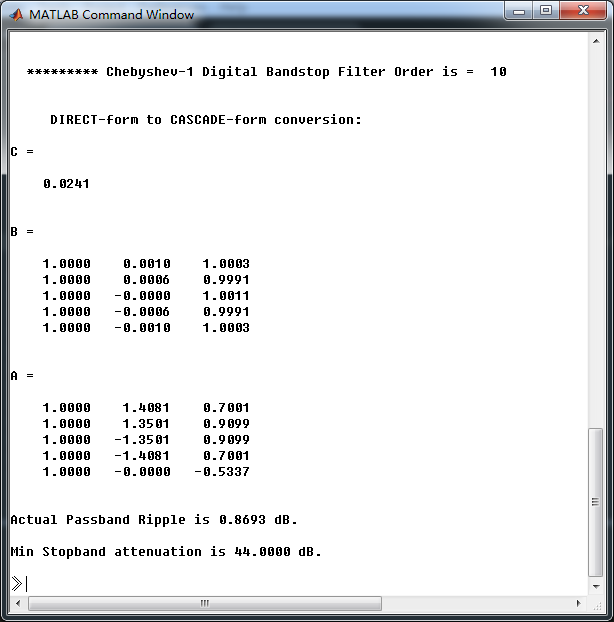
fprintf('\n ********* Chebyshev-1 Digital Bandstop Filter Order is = %3.0f \n', 2*N)
% Digital Chebyshev-1 bandstop Filter Design:
[bbs, abs] = cheby1(N, Rp, wn, 'stop');
[C, B, A] = dir2cas(bbs, abs)
% Calculation of Frequency Response:
[dbbs, magbs, phabs, grdbs, wwbs] = freqz_m(bbs, abs);
% ---------------------------------------------------------------
% find Actual Passband Ripple and Min Stopband attenuation
% ---------------------------------------------------------------
delta_w = 2*pi/1000;
Rp_bs = -(min(dbbs(1:1:ceil(wpbs(1)/delta_w+1)))); % Actual Passband Ripple
fprintf('\nActual Passband Ripple is %.4f dB.\n', Rp_bs);
As_bs = -round(max(dbbs(ceil(wsbs(1)/delta_w)+1:1:ceil(wsbs(2)/delta_w)+1))); % Min Stopband attenuation
fprintf('\nMin Stopband attenuation is %.4f dB.\n\n', As_bs);
%% -----------------------------------------------------------------
%% Plot
%% -----------------------------------------------------------------
figure('NumberTitle', 'off', 'Name', 'Problem 8.40.2 Chebyshev-1 bs by cheby1 function')
set(gcf,'Color','white');
M = 1; % Omega max
subplot(2,2,1); plot(wwbs/pi, magbs); axis([0, M, 0, 1.2]); grid on;
xlabel('Digital frequency in \pi units'); ylabel('|H|'); title('Magnitude Response');
set(gca, 'XTickMode', 'manual', 'XTick', [0, 0.25, 0.35, 0.65, 0.75, M]);
set(gca, 'YTickMode', 'manual', 'YTick', [0, 0.01, 0.9048, 1]);
subplot(2,2,2); plot(wwbs/pi, dbbs); axis([0, M, -120, 2]); grid on;
xlabel('Digital frequency in \pi units'); ylabel('Decibels'); title('Magnitude in dB');
set(gca, 'XTickMode', 'manual', 'XTick', [0, 0.25, 0.35, 0.65, 0.75, M]);
set(gca, 'YTickMode', 'manual', 'YTick', [-80, -44, -1, 0]);
set(gca,'YTickLabelMode','manual','YTickLabel',['80'; '44';'1 ';' 0']);
subplot(2,2,3); plot(wwbs/pi, phabs/pi); axis([0, M, -1.1, 1.1]); grid on;
xlabel('Digital frequency in \pi nuits'); ylabel('radians in \pi units'); title('Phase Response');
set(gca, 'XTickMode', 'manual', 'XTick', [0, 0.25, 0.35, 0.65, 0.75, M]);
set(gca, 'YTickMode', 'manual', 'YTick', [-1:0.5:1]);
subplot(2,2,4); plot(wwbs/pi, grdbs); axis([0, M, 0, 30]); grid on;
xlabel('Digital frequency in \pi units'); ylabel('Samples'); title('Group Delay');
set(gca, 'XTickMode', 'manual', 'XTick', [0, 0.25, 0.35, 0.65, 0.75, M]);
set(gca, 'YTickMode', 'manual', 'YTick', [0:10:30]);
运行结果:
通带、阻带设计指标,dB单位和绝对值单位
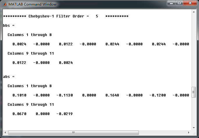
采用cheb1bsf函数,得到Chebyshev-1型数字带阻滤波器,系统函数直接形式的系数如下
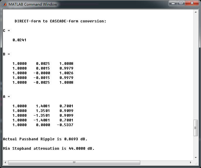
转换成串联形式,系数如下
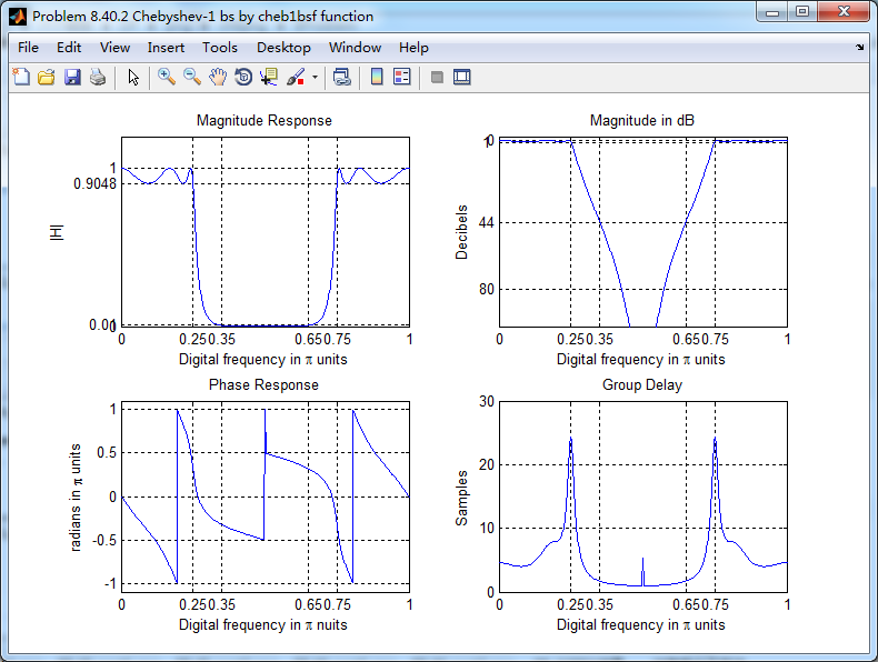
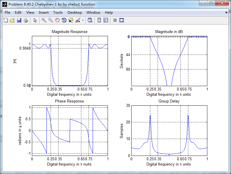
幅度谱、相位谱和群延迟响应
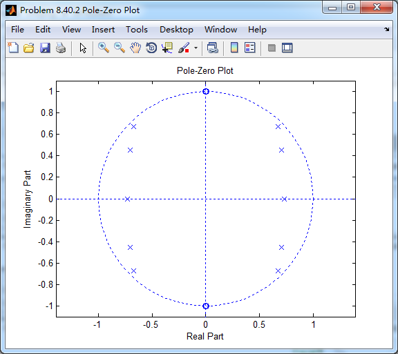
数字带阻滤波器零极点图
和P8.39进行对比,采用cheby1函数(MATLAB工具箱函数),计算得到数字带阻滤波器,系统函数直接形式的系数如下
牢记:
1、如果你决定做某事,那就动手去做;不要受任何人、任何事的干扰。2、这个世界并不完美,但依然值得我们去为之奋斗。

 浙公网安备 33010602011771号