

《DSP using MATLAB》Problem 8.11
代码:
%% ------------------------------------------------------------------------
%% Output Info about this m-file
fprintf('\n***********************************************************\n');
fprintf(' <DSP using MATLAB> Problem 8.11 \n\n');
banner();
%% ------------------------------------------------------------------------
%d = 0.10
%d = 0.05
d = 0.01
a1 = (2-d)/(1+d);
a2 = (2-d)*(1-d)/((2+d)*(1+d));
% digital IIR 2nd-order allpass filter
b = [a2 a1 1]
a = [1 a1 a2]
figure('NumberTitle', 'off', 'Name', 'Problem 8.11 Pole-Zero Plot')
set(gcf,'Color','white');
zplane(b,a);
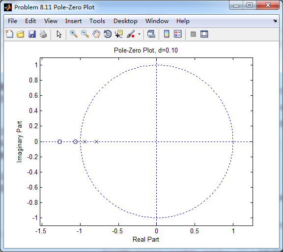
title(sprintf('Pole-Zero Plot, d=%.2f',d));
%pzplotz(b,a);
[db, mag, pha, grd, w] = freqz_m(b, a);
% ---------------------------------------------------------------------
% Choose the gain parameter of the filter, maximum gain is equal to 1
% ---------------------------------------------------------------------
gain1=max(mag) % with poles
K = 1
[db, mag, pha, grd, w] = freqz_m(K*b, a);
figure('NumberTitle', 'off', 'Name', 'Problem 8.11 IIR allpass filter')
set(gcf,'Color','white');
subplot(2,2,1); plot(w/pi, db); grid on; axis([0 2 -60 10]);
set(gca,'YTickMode','manual','YTick',[-60,-30,0])
set(gca,'YTickLabelMode','manual','YTickLabel',['60';'30';' 0']);
set(gca,'XTickMode','manual','XTick',[0,0.25,0.5,1,1.5,1.75,2]);
xlabel('frequency in \pi units'); ylabel('Decibels'); title('Magnitude Response in dB');
subplot(2,2,3); plot(w/pi, mag); grid on; %axis([0 1 -100 10]);
xlabel('frequency in \pi units'); ylabel('Absolute'); title('Magnitude Response in absolute');
set(gca,'XTickMode','manual','XTick',[0,0.25,0.5,1,1.5,1.75,2]);
set(gca,'YTickMode','manual','YTick',[0,1.0]);
subplot(2,2,2); plot(w/pi, pha); grid on; %axis([0 1 -100 10]);
xlabel('frequency in \pi units'); ylabel('Rad'); title('Phase Response in Radians');
subplot(2,2,4); plot(w/pi, grd*pi/180); grid on; %axis([0 1 -100 10]);
xlabel('frequency in \pi units'); ylabel('Rad'); title('Group Delay');
set(gca,'XTickMode','manual','XTick',[0,0.25,0.5,1,1.5,1.75,2]);
%set(gca,'YTickMode','manual','YTick',[0,1.0]);
figure('NumberTitle', 'off', 'Name', 'Problem 8.11 IIR allpass filter')
set(gcf,'Color','white');
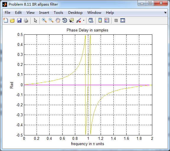
plot(w/pi, -pha/w); grid on; %axis([0 1 -100 10]);
xlabel('frequency in \pi units'); ylabel('Rad'); title('Phase Delay in samples');
% Impulse Response
fprintf('\n----------------------------------');
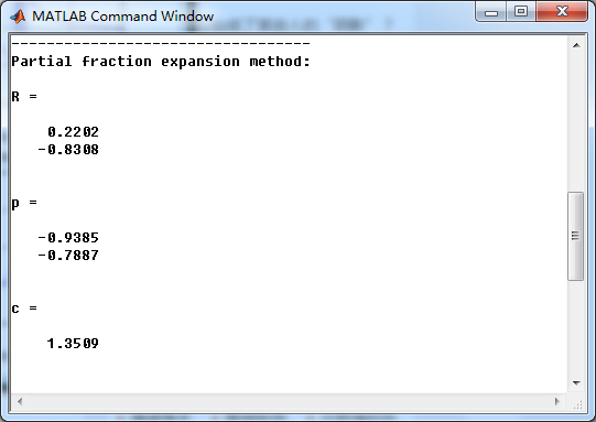
fprintf('\nPartial fraction expansion method: \n');
[R, p, c] = residuez(K*b,a)
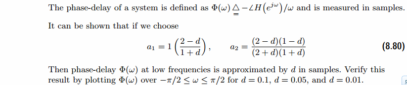
MR = (abs(R))' % Residue Magnitude
AR = (angle(R))'/pi % Residue angles in pi units
Mp = (abs(p))' % pole Magnitude
Ap = (angle(p))'/pi % pole angles in pi units
[delta, n] = impseq(0,0,20);
h_chk = filter(K*b,a,delta); % check sequences
% ------------------------------------------------------------------------------------------------
% gain parameter K
% ------------------------------------------------------------------------------------------------
%h = 0.2202 * ((-0.9385) .^ n) + (-0.8308) * ((-0.7887) .^ n) + 1.3509 * delta; %d=0.1
%h = 0.1099 * ((-0.9688) .^ n) + (-0.4112) * ((-0.8884) .^ n) + 1.1619 * delta; %d=0.05
h = 0.0220 * ((-0.9937) .^ n) + (-0.0820) * ((-0.9766) .^ n) + 1.0305 * delta; %d=0.01
% ------------------------------------------------------------------------------------------------
figure('NumberTitle', 'off', 'Name', 'Problem 8.11 IIR allpass filter, h(n) by filter and Inv-Z ')
set(gcf,'Color','white');
subplot(2,1,1); stem(n, h_chk); grid on; %axis([0 2 -60 10]);
xlabel('n'); ylabel('h\_chk'); title('Impulse Response sequences by filter');
subplot(2,1,2); stem(n, h); grid on; %axis([0 1 -100 10]);
xlabel('n'); ylabel('h'); title('Impulse Response sequences by Inv-Z');
[db, mag, pha, grd, w] = freqz_m(h, [1]);
figure('NumberTitle', 'off', 'Name', 'Problem 8.11 IIR filter, h(n) by Inv-Z ')
set(gcf,'Color','white');
subplot(2,2,1); plot(w/pi, db); grid on; axis([0 2 -60 10]);
set(gca,'YTickMode','manual','YTick',[-60,-30,0])
set(gca,'YTickLabelMode','manual','YTickLabel',['60';'30';' 0']);
set(gca,'XTickMode','manual','XTick',[0,0.25,1,1.75,2]);
xlabel('frequency in \pi units'); ylabel('Decibels'); title('Magnitude Response in dB');
subplot(2,2,3); plot(w/pi, mag); grid on; %axis([0 1 -100 10]);
xlabel('frequency in \pi units'); ylabel('Absolute'); title('Magnitude Response in absolute');
set(gca,'XTickMode','manual','XTick',[0,0.25,1,1.75,2]);
set(gca,'YTickMode','manual','YTick',[0,1.0]);
subplot(2,2,2); plot(w/pi, pha); grid on; %axis([0 1 -100 10]);
xlabel('frequency in \pi units'); ylabel('Rad'); title('Phase Response in Radians');
subplot(2,2,4); plot(w/pi, grd*pi/180); grid on; %axis([0 1 -100 10]);
xlabel('frequency in \pi units'); ylabel('Rad'); title('Group Delay');
set(gca,'XTickMode','manual','XTick',[0,0.25,1,1.75,2]);
%set(gca,'YTickMode','manual','YTick',[0,1.0]);
运行结果:
这里放d=0.1的运行结果。
二阶全通滤波器的留数、极点
系统零极点图,可以看出,两个零点都在单位圆外,幅角为π
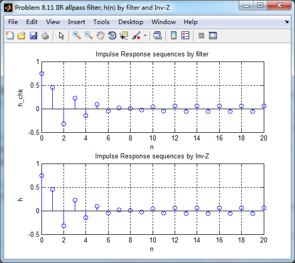
方法一,利用系统函数直接形式,将脉冲序列做输入,得到脉冲响应h,得到系统幅度谱、相位谱和群延迟,如下图

方法二,将二阶全通系统函数部分分式展开,然后查表求逆z变换,得到脉冲响应h_chk
幅度谱、相位谱和群延迟,可以看到,ω=π时,幅度有衰减

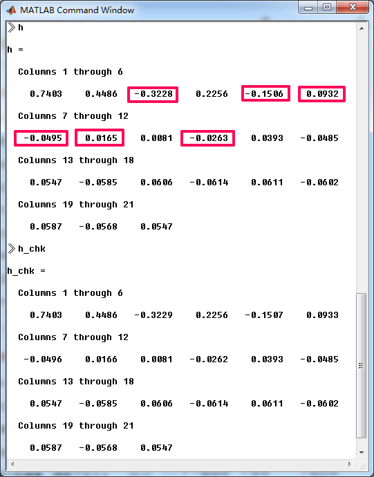
可见,两种方法得到的脉冲响应h有区别,我们将各自前21个元素列出来,方框处二者稍有区别。
但,为何有区别,没搞懂,欢迎各位博友不吝赐教。
牢记:
1、如果你决定做某事,那就动手去做;不要受任何人、任何事的干扰。2、这个世界并不完美,但依然值得我们去为之奋斗。

 浙公网安备 33010602011771号