

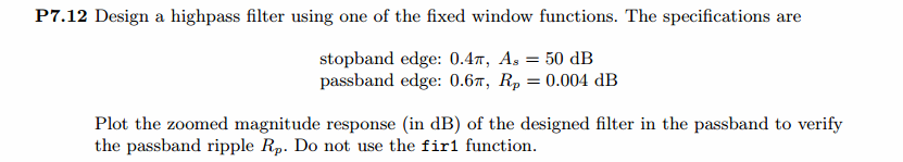
《DSP using MATLAB》Problem 7.12
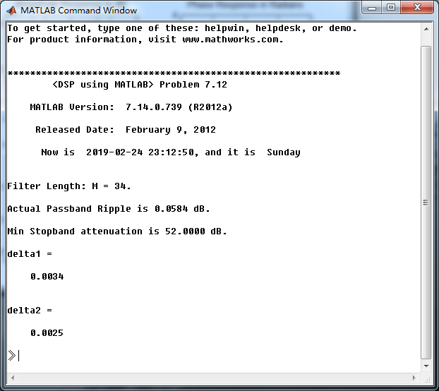
阻带衰减50dB,我们选Hamming窗
代码:
%% ++++++++++++++++++++++++++++++++++++++++++++++++++++++++++++++++++++++++++++++++
%% Output Info about this m-file
fprintf('\n***********************************************************\n');
fprintf(' <DSP using MATLAB> Problem 7.12 \n\n');
banner();
%% ++++++++++++++++++++++++++++++++++++++++++++++++++++++++++++++++++++++++++++++++
% highpass
ws1 = 0.4*pi; wp1 = 0.6*pi; As = 50; Rp = 0.004;
tr_width = (wp1-ws1);
M = ceil(6.6*pi/tr_width) + 1; % Hamming Window
fprintf('\nFilter Length: M = %d.\n', M);
n = [0:1:M-1]; wc1 = (ws1+wp1)/2;
%wc = (ws + wp)/2, % ideal LPF cutoff frequency
hd = ideal_lp(pi, M) - ideal_lp(wc1, M);
w_hamm = (hamming(M))'; h = hd .* w_hamm;
[db, mag, pha, grd, w] = freqz_m(h, [1]); delta_w = 2*pi/1000;
[Hr,ww,P,L] = ampl_res(h);
Rp = -(min(db(wp1/delta_w+1 :1: 0.9*pi/delta_w))); % Actual Passband Ripple
fprintf('\nActual Passband Ripple is %.4f dB.\n', Rp);
As = -round(max(db(1 :1: ws1/delta_w+1 ))); % Min Stopband attenuation
fprintf('\nMin Stopband attenuation is %.4f dB.\n', As);
[delta1, delta2] = db2delta(Rp, As)
% Plot
figure('NumberTitle', 'off', 'Name', 'Problem 7.12 ideal_lp Method')
set(gcf,'Color','white');
subplot(2,2,1); stem(n, hd); axis([0 M-1 -0.4 0.3]); grid on;
xlabel('n'); ylabel('hd(n)'); title('Ideal Impulse Response');
subplot(2,2,2); stem(n, w_hamm); axis([0 M-1 0 1.1]); grid on;
xlabel('n'); ylabel('w(n)'); title('Hamming Window');
subplot(2,2,3); stem(n, h); axis([0 M-1 -0.4 0.3]); grid on;
xlabel('n'); ylabel('h(n)'); title('Actual Impulse Response');
subplot(2,2,4); plot(w/pi, db); axis([0 1 -100 10]); grid on;
set(gca,'YTickMode','manual','YTick',[-90,-52,0]);
set(gca,'YTickLabelMode','manual','YTickLabel',['90';'52';' 0']);
set(gca,'XTickMode','manual','XTick',[0,0.4,0.6,1]);
xlabel('frequency in \pi units'); ylabel('Decibels'); title('Magnitude Response in dB');
figure('NumberTitle', 'off', 'Name', 'Problem 7.12 h(n) ideal_lp Method')
set(gcf,'Color','white');
subplot(2,2,1); plot(w/pi, db); grid on; axis([0 2 -100 10]);
xlabel('frequency in \pi units'); ylabel('Decibels'); title('Magnitude Response in dB');
set(gca,'YTickMode','manual','YTick',[-90,-52,0])
set(gca,'YTickLabelMode','manual','YTickLabel',['90';'52';' 0']);
set(gca,'XTickMode','manual','XTick',[0,0.4,0.6,1,1.4,1.6,2]);
subplot(2,2,3); plot(w/pi, mag); grid on; %axis([0 2 -100 10]);
xlabel('frequency in \pi units'); ylabel('Absolute'); title('Magnitude Response in absolute');
set(gca,'XTickMode','manual','XTick',[0,0.4,0.6,1,1.4,1.6,2]);
set(gca,'YTickMode','manual','YTick',[0.0,0.5,1.0])
subplot(2,2,2); plot(w/pi, pha); grid on; %axis([0 1 -100 10]);
xlabel('frequency in \pi units'); ylabel('Rad'); title('Phase Response in Radians');
subplot(2,2,4); plot(w/pi, grd*pi/180); grid on; %axis([0 1 -100 10]);
xlabel('frequency in \pi units'); ylabel('Rad'); title('Group Delay');
figure('NumberTitle', 'off', 'Name', 'Problem 7.12 h(n)')
set(gcf,'Color','white');
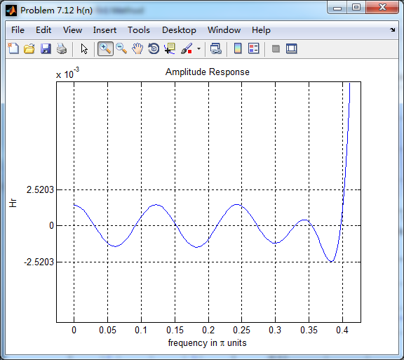
plot(ww/pi, Hr); grid on; %axis([0 1 -100 10]);
xlabel('frequency in \pi units'); ylabel('Hr'); title('Amplitude Response');
set(gca,'YTickMode','manual','YTick',[-delta2,0,delta2,1 - delta1,1, 1 + delta1])
%set(gca,'YTickLabelMode','manual','YTickLabel',['90';'45';' 0']);
%set(gca,'XTickMode','manual','XTick',[0,0.4,0.6,1,1.4,1.6,2]);
h_check = fir1(M, wc1/pi, 'high');
[db, mag, pha, grd, w] = freqz_m(h_check, [1]);
[Hr,ww,P,L] = ampl_res(h_check);
figure('NumberTitle', 'off', 'Name', 'Problem 7.12 fir1 Method')
set(gcf,'Color','white');
subplot(2,2,1); stem(n, hd); axis([0 M-1 -0.4 0.3]); grid on;
xlabel('n'); ylabel('hd(n)'); title('Ideal Impulse Response');
subplot(2,2,2); stem(n, w_hamm); axis([0 M-1 0 1.1]); grid on;
xlabel('n'); ylabel('w(n)'); title('Hanning Window');
subplot(2,2,3); stem([0:M], h_check); axis([0 M -0.4 0.5]); grid on;
xlabel('n'); ylabel('h\_check(n)'); title('Actual Impulse Response');
subplot(2,2,4); plot(w/pi, db); axis([0 1 -100 10]); grid on;
set(gca,'YTickMode','manual','YTick',[-90,-52,0])
set(gca,'YTickLabelMode','manual','YTickLabel',['90';'52';' 0']);
set(gca,'XTickMode','manual','XTick',[0,0.4,0.6,1]);
xlabel('frequency in \pi units'); ylabel('Decibels'); title('Magnitude Response in dB');
figure('NumberTitle', 'off', 'Name', 'Problem 7.12 h(n) fir1 Method')
set(gcf,'Color','white');
subplot(2,2,1); plot(w/pi, db); grid on; axis([0 2 -100 10]);
xlabel('frequency in \pi units'); ylabel('Decibels'); title('Magnitude Response in dB');
set(gca,'YTickMode','manual','YTick',[-90,-52,0])
set(gca,'YTickLabelMode','manual','YTickLabel',['90';'52';' 0']);
set(gca,'XTickMode','manual','XTick',[0,0.4,0.6,1,1.4,1.6,2]);
subplot(2,2,3); plot(w/pi, mag); grid on; %axis([0 1 -100 10]);
xlabel('frequency in \pi units'); ylabel('Absolute'); title('Magnitude Response in absolute');
set(gca,'XTickMode','manual','XTick',[0,0.4,0.6,1,1.4,1.6,2]);
set(gca,'YTickMode','manual','YTick',[0.0,0.5,1.0])
subplot(2,2,2); plot(w/pi, pha); grid on; %axis([0 1 -100 10]);
xlabel('frequency in \pi units'); ylabel('Rad'); title('Phase Response in Radians');
subplot(2,2,4); plot(w/pi, grd*pi/180); grid on; %axis([0 1 -100 10]);
xlabel('frequency in \pi units'); ylabel('Rad'); title('Group Delay');
运行结果:
Hamming窗长度为M=34,实际最小阻带衰减为52dB,满足设计要求。
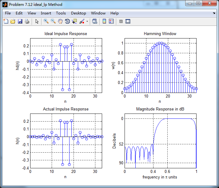
振幅响应的高通部分

低阻部分
下面是用fir1函数(默认Hamming窗)来求得脉冲响应,再计算其幅度响应(dB和Absolute单位)、相位响应和群延迟响应,

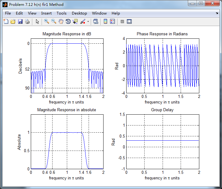
可以看出,两种方法得到的幅度响应和相位响应在接近π的较高频率部分,还是有差别的。
牢记:
1、如果你决定做某事,那就动手去做;不要受任何人、任何事的干扰。2、这个世界并不完美,但依然值得我们去为之奋斗。

 浙公网安备 33010602011771号