反向传播算法

import matplotlib.pyplot as plt
import numpy as np
import seaborn as sns
from sklearn.datasets import make_moons
from sklearn.model_selection import train_test_split
#plt设置
plt.rcParams['font.size']=16
plt.rcParams['font.family']=['STKaiti']
plt.rcParams['axes.unicode_minus']=False
#生成数据集
def load_dataset():
    #采样点数
    N_SAMPLES = 2000
    #测试样本集比例
    TEST_SIZE=0.3
    #生成数据集
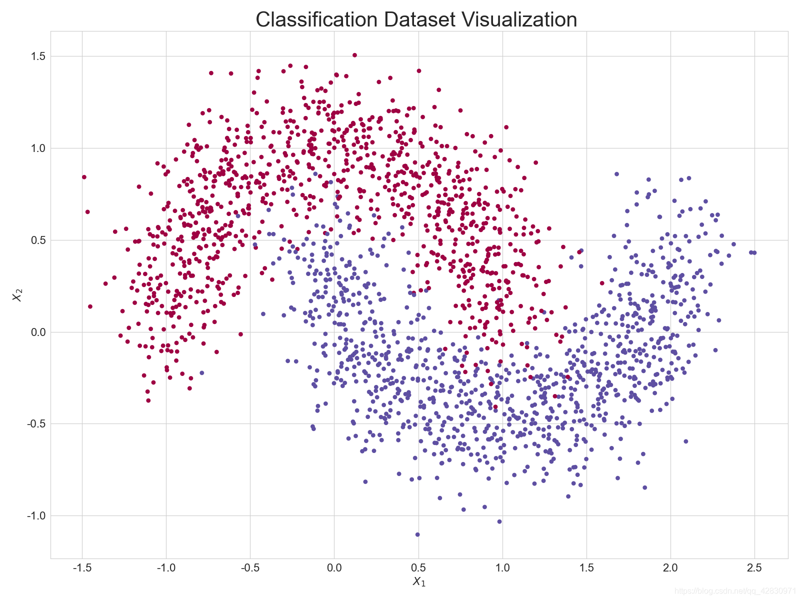
    X,y = make_moons(n_samples = N_SAMPLES,noise = 0.2,random_state = 100)
    #将2000个点分为训练集与测试集，比例0.3
    X_train,X_test,y_train,y_test = train_test_split(X,y,test_size = TEST_SIZE,random_state = 56)
    return X,y,X_train,X_test,y_train,y_test

def make_plot(X,y,plot_name,XX=None,YY=None,preds = None,dark=False):
    #绘制X为坐标，y为标签
    if (dark):
        plt.style.use('dark_background')
    else:
        sns.set_style('whitegrid')
    plt.figure(figsize=(16,12))
    axes = plt.gca()
    axes.set(xlabel='$X_1$',ylabel = '$X_2$')
    plt.title(plot_name,fontsize = 30)
    plt.subplots_adjust(left = 0.2)
    plt.subplots_adjust(right = 0.8)
    if XX is not None and YY is not None and preds is not None:
        plt.contourf(XX,YY,preds.reshape(XX.shape),25,alpha=1,cmap=plt.cm.Spectral)
        plt.contour(XX, YY, preds.reshape(XX.shape), levels=[.5], cmap="Greys", vmin=0, vmax=.6)
    # 绘制散点图，根据标签区分颜色
    plt.scatter(X[:, 0], X[:, 1], c=y.ravel(), s=40, cmap=plt.cm.Spectral, edgecolors='none')
    plt.show()


X, y, X_train, X_test, y_train, y_test = load_dataset()
# 调用 make_plot 函数绘制数据的分布，其中 X 为 2D 坐标， y 为标签
make_plot(X, y, "Classification Dataset Visualization ")

class Layer:
    def __init__(self,n_input,n_neurons,activation = None,weights = None,bias = None):
        self.weights= weights if weights is not None else np.random.randn(n_input,n_neurons) * np.sqrt(1/n_neurons)
        self.bias = bias if bias is not None else np.random.rand(n_neurons) * 0.1
        self.activation = activation
        self.last_activation = None
        self.error = None
        self.delta = None
    def activate(self,x):
        r=np.dot(x,self.weights)+self.bias
        self.last_activation = self._apply_activation(r)
        return self.last_activation
    def _apply_activation(self,r):
        if self.activation is None:
            return r  # 无激活函数，直接返回
        # ReLU 激活函数
        elif self.activation == 'relu':
            return np.maximum(r, 0)
        # tanh 激活函数
        elif self.activation == 'tanh':
            return np.tanh(r)
        # sigmoid 激活函数
        elif self.activation == 'sigmoid':
            return 1 / (1 + np.exp(-r))
        return r
    def apply_activation_derivative(self, r):
        # 计算激活函数的导数
        # 无激活函数，导数为1
        if self.activation is None:
            return np.ones_like(r)
        # ReLU 函数的导数实现
        elif self.activation == 'relu':
            grad = np.array(r, copy=True)
            grad[r > 0] = 1.
            grad[r <= 0] = 0.
            return grad
        # tanh 函数的导数实现
        elif self.activation == 'tanh':
            return 1 - r ** 2
        # Sigmoid 函数的导数实现
        elif self.activation == 'sigmoid':
            return r * (1 - r)
        return r

class NeuralNetwork:
    def __init__(self):
        self._layers =[]
    def add_layer(self,layer):
        self._layers.append(layer)
    def feed_forward(self,X):
        for layer in self._layers:
            X = layer.activate(X)
        return X
    def backpropagation(self, X, y, learning_rate):
        output = self.feed_forward(X)
        for i in reversed(range(len(self._layers))):  # 反向循环
            layer = self._layers[i]  # 得到当前层对象
            # 如果是输出层
            if layer == self._layers[-1]:  # 对于输出层
                layer.error = y - output  # 计算2 分类任务的均方差的导数
                # 关键步骤：计算最后一层的delta，参考输出层的梯度公式
                layer.delta = layer.error * layer.apply_activation_derivative(output)
            else:  # 如果是隐藏层
                next_layer = self._layers[i + 1]  # 得到下一层对象
                layer.error = np.dot(next_layer.weights, next_layer.delta)
                # 关键步骤：计算隐藏层的delta，参考隐藏层的梯度公式
                layer.delta = layer.error * layer.apply_activation_derivative(layer.last_activation)

        # 循环更新权值
        for i in range(len(self._layers)):
            layer = self._layers[i]
            # o_i 为上一网络层的输出
            o_i = np.atleast_2d(X if i == 0 else self._layers[i - 1].last_activation)
            # 梯度下降算法，delta 是公式中的负数，故这里用加号
            layer.weights += layer.delta * o_i.T * learning_rate

    def train(self, X_train, X_test, y_train, y_test, learning_rate, max_epochs):
        # 网络训练函数
        # one-hot 编码
        y_onehot = np.zeros((y_train.shape[0], 2))
        y_onehot[np.arange(y_train.shape[0]), y_train] = 1

        # 将One-hot 编码后的真实标签与网络的输出计算均方误差，并调用反向传播函数更新网络参数，循环迭代训练集1000 遍即可
        mses = []
        accuracys = []
        for i in range(max_epochs + 1):  # 训练1000 个epoch
            for j in range(len(X_train)):  # 一次训练一个样本
                self.backpropagation(X_train[j], y_onehot[j], learning_rate)
            if i % 10 == 0:
                # 打印出MSE Loss
                mse = np.mean(np.square(y_onehot - self.feed_forward(X_train)))
                mses.append(mse)
                accuracy = self.accuracy(self.predict(X_test), y_test.flatten())
                accuracys.append(accuracy)
                print('Epoch: #%s, MSE: %f' % (i, float(mse)))
                # 统计并打印准确率
                print('Accuracy: %.2f%%' % (accuracy * 100))
        return mses, accuracys

    def predict(self, X):
        return self.feed_forward(X)

    def accuracy(self, X, y):
        return np.sum(np.equal(np.argmax(X, axis=1), y)) / y.shape[0]


nn = NeuralNetwork()  # 实例化网络类
nn.add_layer(Layer(2, 25, 'sigmoid'))  # 隐藏层 1, 2=>25
nn.add_layer(Layer(25, 50, 'sigmoid'))  # 隐藏层 2, 25=>50
nn.add_layer(Layer(50, 25, 'sigmoid'))  # 隐藏层 3, 50=>25
nn.add_layer(Layer(25, 2, 'sigmoid'))  # 输出层, 25=>2
mses, accuracys = nn.train(X_train, X_test, y_train, y_test, 0.01, 1000)


x = [i for i in range(0, 101, 10)]

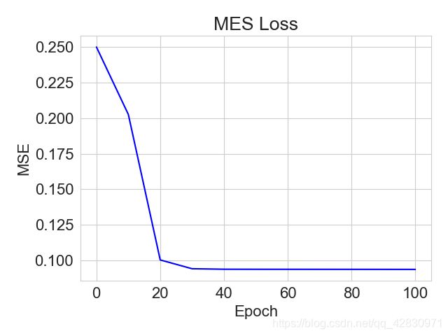
# 绘制MES曲线
plt.title("MES Loss")
plt.plot(x, mses[:11], color='blue')
plt.xlabel('Epoch')
plt.ylabel('MSE')
plt.show()

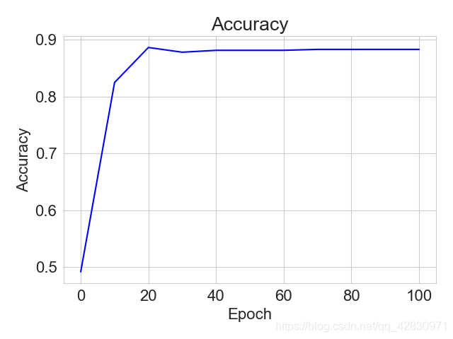
# 绘制Accuracy曲线
plt.title("Accuracy")
plt.plot(x, accuracys[:11], color='blue')
plt.xlabel('Epoch')
plt.ylabel('Accuracy')
plt.show()