
OpenCV直方图(直方图、直方图均衡,直方图匹配,原理、实现)
1 直方图
灰度级范围为 \([0,L-1]\) 的数字图像的直方图是离散函数 \(h(r_k) = n_k\) , 其中 \(r_k\) 是第\(k\)级灰度值,\(n_k\) 是图像中灰度为 \(r_k\) 的像素个数。在实践中,经常用乘积 \(MN\) 表示的图像像素的总数除它的每个分量来归一化直方图,通常 \(M\) 和 \(N\) 是图像的行和列的位数。因此,归一化后的直方图由 \(p(r_k) = n_k/MN\) 给出,其中 \(k = 0, 1, ... ,L-1\) 。简单地说, \(p(r_k)\) 是灰度级 \(r_k\) 在图像中出现的概率的一个估计。归一化直方图的所有分量之和应等于1。
在OPENCV3.0中有相关函数如下,其中有3个版本,这是经常用到的一个:
CV_EXPORTS void calcHist( const Mat* images,
                          int nimages,
                          const int* channels,
                          InputArray mask,
                          OutputArray hist,
                          int dims,
                          const int* histSize,
                          const float** ranges,
                          bool uniform = true,
                          bool accumulate = false );
images, 是要求的Mat的指针,这里可以传递一个数组,可以同时求很多幅图片的直方图,前提是他们的深度相同,CV_8U或者CV_32F,尺寸相同。通道数可以不同;
nimages, 源图像个数;
channels, 传递要加入直方图计算的通道。该函数可以求多个通道的直方图。通道序号从0开始依次递增。假如第一幅图像有3个通道,第二幅图像有两个通道。则:images[0]的通道序号为0、1、2,images[1]的通道序号则为3、4;如果想通过5个通道计算直方图,则传递的通道channels为int channels[5] = {0, 1, 2, 3, 4, 5}。
mask, 掩码矩阵,没有掩码,则传递空矩阵就行了。如果非空则掩码矩阵大小必须和图像大小相同,在掩码矩阵中非空元素将被计算到直方图内。
hist, 输出直方图;
dims, 直方图维度,必须大于0,并小于CV_MAX_DIMS(32);
histSize, 直方图中每个维度级别数量,比如灰度值(0-255),如果级别数量为4,则灰度值直方图会按照[0, 63],[64,127,[128,191],[192,255],也称为bin数目,这里是4个bin。如果是多维的就需要传递多个。每个维度的大小用一个int来表示。所以histSize是一个数组;
ranges, 一个维度中的每一个bin的取值范围。如果uniform == true,则range可以用一个具有2个元素(一个最小值和一个最大值)的数组表示。如果uniform == false,则需要用一个具有histSize + 1个元素(每相邻的两个元素组成的取值空间代表对应的bin的取值范围)的数组表示。如果统计多个维度则需要传递多个数组。所以ranges,是一个二维数组。如下代码是uniform == false时的情况:
int nHistSize[] = { 5 };
// range有6个元素,每个元素,组成5个bin的取值范围
float range[] = { 0, 70,100, 120, 200,255 };
const float* fHistRanges[] = { range };
Mat histR, histG, histB;
// 这里的uniform == false
calcHist(&matRGB[1], 1, &nChannels, Mat(), histB, 1, nHistSize, fHistRanges, false, false);
uniform, 表示直方图中一个维度中的各个bin的宽度是否相同或,详细解释见ranges中介绍;
accumulate, 在计算直方图时是否清空传入的hist。true,则表示不清空,false表示清空。该参数一般设置为false。只有在想要统计多个图像序列中的累加直方图时才会设置为true。例如:
calcHist(mat1, 1, &nChannels, Mat(), hist, 1, nHistSize, fHistRanges, true, false);
calcHist(mat2, 1, &nChannels, Mat(), hist, 1, nHistSize, fHistRanges, true, true);
以上代码统计了mat1和mat2中图像数据的直方图到hist中。也就是说hist中的直方图数据是从matRGB1和mat2中统计出来的,不单单是mat1的数据,也不单单是mat2的数据。如果第二行中最后一个参数为false则hist中统计的数据单单是mat2的,mat1的数据被清空了。
1.1 统计灰度直方图
#include "opencv2/core/core.hpp"
#include "opencv2/imgproc/imgproc.hpp"
#include "opencv2/highgui/highgui.hpp"
#include <string>
using namespace cv;
int main()
{
std::string strPath = "D:\\MyDocuments\\My Pictures\\OpenCV\\";
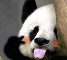
Mat matSrc = imread(strPath + "panda.jpg");
Mat matRGB[3];
split(matSrc, matRGB);
int Channels[] = { 0 };
int nHistSize[] = { 256 };
float range[] = { 0, 255 };
const float* fHistRanges[] = { range };
Mat histR, histG, histB;
// 计算直方图
calcHist(&matRGB[0], 1, Channels, Mat(), histB, 1, nHistSize, fHistRanges, true, false);
calcHist(&matRGB[1], 1, Channels, Mat(), histG, 1, nHistSize, fHistRanges, true, false);
calcHist(&matRGB[2], 1, Channels, Mat(), histR, 1, nHistSize, fHistRanges, true, false);
// 创建直方图画布
int nHistWidth = 800;
int nHistHeight = 600;
int nBinWidth = cvRound((double)nHistWidth / nHistSize[0]);
Mat matHistImage(nHistHeight, nHistWidth, CV_8UC3, Scalar(255, 255, 255));
// 直方图归一化
normalize(histB, histB, 0.0, matHistImage.rows, NORM_MINMAX, -1, Mat());
normalize(histG, histG, 0.0, matHistImage.rows, NORM_MINMAX, -1, Mat());
normalize(histR, histR, 0.0, matHistImage.rows, NORM_MINMAX, -1, Mat());
// 在直方图中画出直方图
for (int i = 1; i < nHistSize[0]; i++)
{
line(matHistImage,
Point(nBinWidth * (i - 1), nHistHeight - cvRound(histB.at<float>(i - 1))),
Point(nBinWidth * (i), nHistHeight - cvRound(histB.at<float>(i))),
Scalar(255, 0, 0),
2,
8,
0);
line(matHistImage,
Point(nBinWidth * (i - 1), nHistHeight - cvRound(histG.at<float>(i - 1))),
Point(nBinWidth * (i), nHistHeight - cvRound(histG.at<float>(i))),
Scalar(0, 255, 0),
2,
8,
0);
line(matHistImage,
Point(nBinWidth * (i - 1), nHistHeight - cvRound(histR.at<float>(i - 1))),
Point(nBinWidth * (i), nHistHeight - cvRound(histR.at<float>(i))),
Scalar(0, 0, 255),
2,
8,
0);
}
// 显示直方图
imshow("histogram", matHistImage);
imwrite(strPath + "histogram.jpg", matHistImage);
waitKey();
return 0;
}
原图:
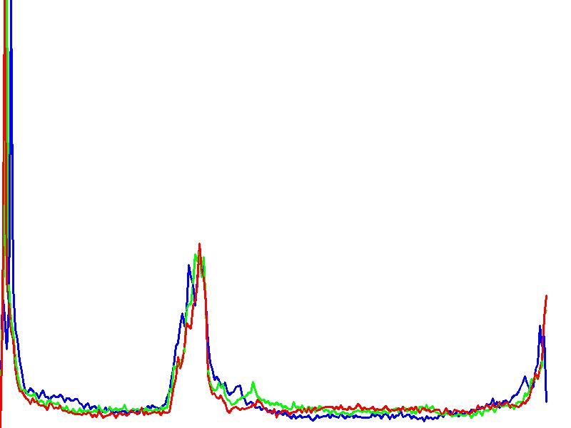
直方图:
1.2 H-S直方图
H-S直方图是图片再HSV空间中,统计的H和S两个维度的直方图。代码如下:
#include "opencv2/core/core.hpp"
#include "opencv2/imgproc/imgproc.hpp"
#include "opencv2/highgui/highgui.hpp"
#include <string>

using namespace cv;

int main()
{
    Mat matSrc, matHsv;
    std::string strPath = "D:\\MyDocuments\\My Pictures\\OpenCV\\";
    matSrc = imread(strPath + "panda_mini.jpg");
    if (matSrc.empty())
        return -1;
    cvtColor(matSrc, matHsv, CV_BGR2HSV);

    int nRows = matSrc.rows;
    int nCols = matSrc.cols;
    std::cout << nRows << std::endl;
    std::cout << nCols << std::endl;

    int hbins = 30, sbins = 32;
    int histSize[] = { hbins, sbins };
    float hranges[] = { 0, 180 };
    float sranges[] = { 0, 256 };
    const float * ranges[] = { hranges, sranges };
    Mat hist;

    int channels[] = { 0, 1 };
    calcHist(&matHsv, 1, channels, Mat(), hist, 2, histSize, ranges, true, false);

    double  maxVal = 0;
    minMaxLoc(hist, 0, &maxVal, 0, 0);
    int nScale = 10;

    Mat histImg = Mat::zeros(sbins * nScale, hbins * nScale, CV_8UC3);
    // 遍历H、S通道
    for (int j = 0; j < hbins; j++)
    {
        for (int i = 0; i < sbins; i++)
        {
            float binVal = hist.at<float>(j, i);
            // 根据最大值计算变化范围
            int intensity = cvRound(binVal * 255 / maxVal);
            // 绘图显示
            rectangle(histImg,
                Point(j * nScale, i * nScale),
                Point((j + 1) * nScale - 1, (i + 1) * nScale - 1),
                Scalar::all(intensity),
                CV_FILLED);
        }
    }
    imshow("src", matSrc);
    imshow("h-s", histImg);
    waitKey();
    return 0;
}
原图: 
直方图: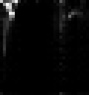
1.3 统计uniform = false的直方图
#include "opencv2/core/core.hpp"
#include "opencv2/imgproc/imgproc.hpp"
#include "opencv2/highgui/highgui.hpp"
#include <string>

using namespace cv;

bool histImage(Mat &hist, Mat &matHistImage, int width, int height, int binWidth, int type, Scalar color);

int main()
{
    std::string strPath = "D:\\MyDocuments\\My Pictures\\OpenCV\\";
    Mat matSrc = imread(strPath + "panda.jpg", 1);

    int nChannels = 0;
    int Channels[] = { 0 };
    int nHistSize[] = { 5 };
    float range[] = { 0, 70,100, 120, 200,255 }; // 数组中有nHistSize[0] + 1个元素
    const float* fHistRanges[] = { range };
    Mat hist;
    // 计算直方图,uniform = false
    calcHist(&matSrc, 1, Channels, Mat(), histB, 1, nHistSize, fHistRanges, false, false);
    // 创建直方图画布
    int nHistWidth = 800;
    int nHistHeight = 600;
    int nBinWidth = cvRound((double)nHistWidth / nHistSize[0]);
    // 直方图归一化
    normalize(histB, histB, 0.0, nHistHeight, NORM_MINMAX, -1, Mat());
    // 在直方图中画出直方图
    Mat matHistImage;
    histImage(histB, matHistImage, nHistWidth, nHistHeight, nBinWidth, CV_8UC3, Scalar(255, 0, 0));
    // 显示直方图
    imshow("histogram", matHistImage);
    imwrite(strPath + "panda_histogram_uniform_false.jpg", matHistImage);
    waitKey();
    return 0;
}

bool histImage(Mat &hist, Mat &matHistImage, int width, int height, int binWidth, int type, Scalar color)
{
    if (2 != hist.dims)
        return false;
    if (matHistImage.empty())
    {
        matHistImage.create(height, width, type);
    }
    for (int i = 1; i < hist.rows; i++)
    {
        line(matHistImage,
            Point(binWidth * (i - 1), height - cvRound(hist.at<float>(i - 1))),
            Point(binWidth * (i), height - cvRound(hist.at<float>(i))),
            color,
            2,
            8,
            0);
    }
}
原图:

直方图:

2 直方图均衡
我们很难观察一幅非常亮或暗的图像的细节信息,因此对于差异较较大的图像,我们可以尝试改变图像灰度分布来使图像灰度阶分布尽量均匀,进而增强图像细节信息。我们先考虑连续灰度值的情况,用变量 \(r\) 表示待处理图像的灰度。假设 \(r\) 的取值范围为 \([0, L-1]\) ,且 \(r = 0\) 表示黑色, \(r = L-1\) 表示白色。在 \(r\) 满足这些条件的情况下,我们注意里几种在变换形式
我们假设:
(a) \(T(r)\) 在区间 \(0 \leq r \leq L-1\) 上为严格单调递增函数。
(b) 当 \(0 \leq r \leq L-1\) 时, \(0 \leq T(r) \leq L-1\) 。
则:
一幅图像的灰度值可以看成是区间 \([0, L-1]\) 内的随机变量。随机变量的基本描绘是器概率密度函数。令 \(p_r(r)\) 和 \(p_s(s)\) 分别表示变量 \(r\) 和 \(s\) 的概率密度函数,其中 \(p\) 的下标用于指示 \(p_r\) 和 \(p_s\) 是不同的函数。有基本概率论得到的一个基本结果是,如果 \(p_r(r)\) 和 \(T(r)\) 已知,且在感兴趣的值域上 \(T(r)\) 是连续且可微的, 则变换(映射)后的变量 \(s\) 的概率密度函数如下:
这样,我们看到,输出灰度变量s的概率密度函数是由变换函数 \(T(r)\) 决定的。而在图像处理中特别重要的也比较常用的变化如下:
其中,\(w\) 是假积分变量。公式右边是随机变量 \(r\) 的累计分布函数。因为概率密度函数总为正,一个函数的积分是该函数下方的面积。则上式子则满足(a)条件,当 \(r = L-1\) 时,则积分值等于1,所以 \(s\) 的最大值是 \(L-1\),所以上式满足条件(b).
而:
带入(1)得:
由 \(p_s(s)\) 可知,这是一个均匀概率密度函数。简而言之,(2)中的变换将得到一个随机变量 \(s\) ,该随机变量有一个均匀的概率密度函数表征。而 \(p_s(s)\) 始终是均匀的,它于 \(p_r(r)\) 的形式无关。
对于离散值,我们处理其概率(直方图值)与求和来替代处理概率密度函数与积分。则一幅数字图像中灰度级 \(r_k\) 出现的概率近似为
其中,\(MN\)是图像中像素的总数,\(n_k\) 是灰度为 \(r_k\) 的像素个数, \(L\) 是图像中可能的灰度级的数量(8bit图像时256)。与 \(r_k\) 相对的 \(p_r(r_k)\)图形通常称为直方图。
式(2)的离散形式为
在OPENCV中由实现直方图均衡化的函数:
void equalizeHist( InputArray src, OutputArray dst );
示例代码:
#include "opencv2/core/core.hpp"
#include "opencv2/imgproc/imgproc.hpp"
#include "opencv2/highgui/highgui.hpp"
#include <iostream>
#include <string>

using namespace cv;

int equalizeHist();
int equalizeHist_Color();


int main()
{
    equalizeHist();
    equalizeHist_Color();
    cvWaitKey();
    return 0;
}

int equalizeHist()
{
    std::string strPath = "D:\\MyDocuments\\My Pictures\\OpenCV\\";
    Mat matSrc = imread(strPath + "pic2.jpg");
    if (matSrc.empty())
    {
        return -1;
    }
    imshow("src", matSrc);
    Mat matGray;
    cvtColor(matSrc, matGray, CV_BGR2GRAY);
    // 直方图均衡化
    Mat matResult;
    equalizeHist(matGray, matResult);

    imshow("equlizeHist", matResult);
    imwrite(strPath + "pic2_gray.jpg", matGray);
    imwrite(strPath + "pic2_equlizeHist.jpg", matResult);
    return 0;
}

int equalizeHist_Color()
{
    std::string strPath = "D:\\MyDocuments\\My Pictures\\OpenCV\\";
    Mat matSrc = imread(strPath + "pic2.jpg");
    if (matSrc.empty())
    {
        return -1;
    }
    Mat matArray[3];
    split(matSrc, matArray);
    // 直方图均衡化
    for (int i = 0; i < 3; i++)
    {
        equalizeHist(matArray[i], matArray[i]);
    }
    Mat matResult;
    merge(matArray, 3, matResult);


    imshow("src", matSrc);
    imshow("equlizeHist", matResult);

    imwrite(strPath + "pic2_equlizeHist_color.jpg", matResult);
    return 0;
}
原图:

灰度图:
灰度图均衡直方图后:
彩色图均衡直方图后:

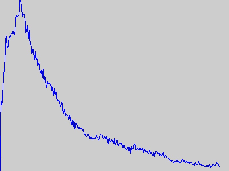
灰度图均衡前直方图
灰度图均衡直方图后的直方图:
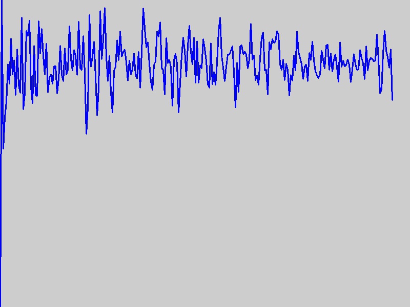
我们可以看到均衡直方图后的直方图比较相对来说比较均匀了。不过可以看出均衡直方图后的图像的直方图并不是像标准的均匀分布。这是因为我们在推导的是把灰度值看成连续的才会有(3)式的结果。也就是说直方图其实是概率密度函数的近似,我们实际上是把连续的灰度级强制的映射到了有限的离散的灰度级上。并且在处理中不允许又新的灰度级产生。所以在实际的直方图均衡应用中,很少见到完美平坦的直方图。
3 直方图匹配
在实际场景中,我们常常需要增强某一特定区间的图像信息,对于某些应用,采用均匀直方图的基本增强并不是最好的方法。有时我们希望处理后的图像具有规定的直方图形状可能更有用。这种用于产生处理后又特殊直方图的方法称为直方图匹配或直方图规定化。
继续用连续灰度 \(r\) 、\(z\)、\(s\),并令 \(p_r(r)\) 和 \(p_z(z)\) 表示它们所对应的连续概率密度函数。在这种表示方法中, \(r\) 和 \(z\) 分别表示输入图像和输出(已处理)图像的灰度级。我们可以由给定的输入图像估计 \(p_r(r)\), 而 \(p_z(z)\)是我们希望输出图像所具有的指定概率密度函数。
令 \(s\) 为一个有如下特性的随机变量:
其中,如前面一样,\(w\) 为积分假变量。这个表达式是直方图均衡的连续形式。
接着,我们定义一个有如下特性的随机变量 \(z\):
其中,\(t\) 为积分假变量。由式(4)和式(5)可得, \(G(z) = T(r)\),因此 \(z\)必须满足以下条件:
一旦由输入图像估计出 \(p_r(r)\), 变换函数 \(T(r)\)就可由式(4)得到。类似地,因为 \(p_z(z)\),已知,变换函数 \(G(z)\) 可由式(5)得到。
式(4)到式(6)表明,使用下列步骤,可由一幅给定图像得到一幅其灰度级具有指定概率密度函数的图像:
1、由输入图像得到 \(p_r(r)\), 并由式(4)求得 \(s\) 的值;
2、使用式(11)中指定的概率密度函数求的变换函数 \(G(z)\);
3、求的变换函数 \(z = G{-1}(s)\); 因为 \(z\) 是由 \(s\) 得到的,所以该处理是 \(s\) 到 \(z\)的映射,而后者正是我们期望的值;
4、首先用式(4)对输入头像均衡得到输出图像;该图像的像素值是 \(s\) 值。对均衡就后的图像中具有 \(s\) 值的每个像素执行反映射 \(z = G^{-1}(s)\),得到输出图像中的相应像素。当所以的像素都处理完后,输出图像的概率密度函数将等于指定的概率密度函数。
如直方图均衡中一样,直方图规定话在原理上是简单的。在实际中的困难是寻找 \(T(r)\) 和 \(G^{-1}\) 的有意义的表达式。不过我们是在离散情况下的,则问题可以简化很多。式(4)的离散形式如下:
其中 \(MN\) 式图像的像素总数, \(n_j\) 是具有灰度值 \(r_j\) 的像素数, \(L\) 是图像中可能的灰度级数。类似的,给定一个规定的 \(s_k\) 值, 式(5)的离散形式设计计算变化函数
对一个 \(q\) 值,有
其中, \(p_z(z_i)\) 时规定的直方图的第 \(i\) 个值。 方便换找到期望的值 \(z_q\):
也就是说,该操作对每一个 \(s\) 值给出一个 \(z\) 值;这样就形成了从 \(s\) 到 \(z\) 的映射。
我们不需要计算 \(G\) 的反变换。因为我们处理的灰度级是整数(如8bit图像的灰度级从0到255),通过式(7)可以容易地计算 \(q = 0,1,3,...,L-1\) 所有可能的 \(G\) 值。标定这些值,并四舍五入为区间 \([0, L-1]\) 内的最接近整数。将这些值存储在一个表中。然后给定一个特殊的 \(s_k\) 值后,我们可以查找存储在表中的最匹配的值。这样,给定的 \(s_k\) 值就与相应的 \(z\) 值关联在一起了。这样能找到每个 \(s_k\) 值到 \(z_q\) 值的映射。也就是式(8)的近似。这些映射也是直方图规定化问题的解。
这里还有个问题,就是在离散情况下,式(7)不再式严格单调的,则式(9)可能会出现一对多的映射,还有可能出现有些值没有映射的情况。这里采用的办法式对于一对多的情况做个平均(因为式(7)可能不在严格单调,但仍然是单调不减的,所以平均很合适),对于没有映射的则取其最接近的值。
示例代码:
#include "opencv2/core/core.hpp"
#include "opencv2/imgproc/imgproc.hpp"
#include "opencv2/highgui/highgui.hpp"
#include <iostream>
#include <string>

using namespace cv;

bool histMatch_Value(Mat matSrc, Mat matDst, Mat &matRet);
int histogram_Matching();

int main()
{
    histogram_Matching();
    return 0;
}

bool histMatch_Value(Mat matSrc, Mat matDst, Mat &matRet)
{
    if (matSrc.empty() || matDst.empty() || 1 != matSrc.channels() || 1 != matDst.channels())
        return false;
    int nHeight = matDst.rows;
    int nWidth = matDst.cols;
    int nDstPixNum = nHeight * nWidth;
    int nSrcPixNum = 0;

    int arraySrcNum[256] = { 0 };                // 源图像各灰度统计个数
    int arrayDstNum[256] = { 0 };                // 目标图像个灰度统计个数
    double arraySrcProbability[256] = { 0.0 };   // 源图像各个灰度概率
    double arrayDstProbability[256] = { 0.0 };   // 目标图像各个灰度概率
    // 统计源图像
    for (int j = 0; j < nHeight; j++)
    {
        for (int i = 0; i < nWidth; i++)
        {
            arrayDstNum[matDst.at<uchar>(j, i)]++;
        }
    }
    // 统计目标图像
    nHeight = matSrc.rows;
    nWidth = matSrc.cols;
    nSrcPixNum = nHeight * nWidth;
    for (int j = 0; j < nHeight; j++)
    {
        for (int i = 0; i < nWidth; i++)
        {
            arraySrcNum[matSrc.at<uchar>(j, i)]++;
        }
    }
    // 计算概率
    for (int i = 0; i < 256; i++)
    {
        arraySrcProbability[i] = (double)(1.0 * arraySrcNum[i] / nSrcPixNum);
        arrayDstProbability[i] = (double)(1.0 * arrayDstNum[i] / nDstPixNum);
    }
    // 构建直方图均衡映射
    int L = 256;
    int arraySrcMap[256] = { 0 };
    int arrayDstMap[256] = { 0 };
    for (int i = 0; i < L; i++)
    {
        double dSrcTemp = 0.0;
        double dDstTemp = 0.0;
        for (int j = 0; j <= i; j++)
        {
            dSrcTemp += arraySrcProbability[j];
            dDstTemp += arrayDstProbability[j];
        }
        arraySrcMap[i] = (int)((L - 1) * dSrcTemp + 0.5);// 减去1,然后四舍五入
        arrayDstMap[i] = (int)((L - 1) * dDstTemp + 0.5);// 减去1,然后四舍五入
    }
    // 构建直方图匹配灰度映射
    int grayMatchMap[256] = { 0 };
    for (int i = 0; i < L; i++) // i表示源图像灰度值
    {
        int nValue = 0;    // 记录映射后的灰度值
        int nValue_1 = 0;  // 记录如果没有找到相应的灰度值时,最接近的灰度值
        int k = 0;
        int nTemp = arraySrcMap[i];
        for (int j = 0; j < L; j++) // j表示目标图像灰度值
        {
            // 因为在离散情况下,之风图均衡化函数已经不是严格单调的了,
            // 所以反函数可能出现一对多的情况,所以这里做个平均。
            if (nTemp == arrayDstMap[j])
            {
                nValue += j;
                k++;
            }
            if (nTemp < arrayDstMap[j])
            {
                nValue_1 = j;
                break;
            }
        }
        if (k == 0)// 离散情况下,反函数可能有些值找不到相对应的,这里去最接近的一个值
        {
            nValue = nValue_1;
            k = 1;
        }
        grayMatchMap[i] = nValue/k;
    }
    // 构建新图像
    matRet = Mat::zeros(nHeight, nWidth, CV_8UC1);
    for (int j = 0; j < nHeight; j++)
    {
        for (int i = 0; i < nWidth; i++)
        {
            matRet.at<uchar>(j, i) = grayMatchMap[matSrc.at<uchar>(j, i)];
        }
    }
    return true;
}

int histogram_Matching()
{
    std::string strPath = "D:\\MyDocuments\\My Pictures\\OpenCV\\";
    Mat matSrc = imread(strPath + "pic2.jpg"); // 源图像
    Mat matDst = imread(strPath + "pic3.jpg"); // 目标图像

    Mat srcBGR[3];
    Mat dstBGR[3];
    Mat retBGR[3];
    split(matSrc, srcBGR);
    split(matDst, dstBGR);

    histMatch_Value(srcBGR[0], dstBGR[0], retBGR[0]);
    histMatch_Value(srcBGR[1], dstBGR[1], retBGR[1]);
    histMatch_Value(srcBGR[2], dstBGR[2], retBGR[2]);

    Mat matResult;
    merge(retBGR, 3, matResult);
    imshow("src", matSrc);
    imshow("dst", matDst);
    imshow("Ret", matResult);

    imwrite(strPath + "hist_match_value.jpg", matResult);

    cvWaitKey();
    return 0;
}
原图:

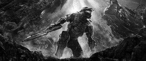
目标图:

原图按照目标图直方图匹配后:

直方图匹配和均衡直方图效果还是有很多差别的,感兴趣的可以和前面的均衡直方图比较一下。直方图匹配可以说是把一幅图转换成另一幅的风格。

 浙公网安备 33010602011771号