【论文阅读】RAL 2022: Receding Moving Object Segmentation in 3D LiDAR Data Using Sparse 4D Convolutions
参考与前言
Status: Finished
Type: RAL
Year: 2022
论文链接:https://www.ipb.uni-bonn.de/wp-content/papercite-data/pdf/mersch2022ral.pdf
代码链接:https://github.com/PRBonn/4DMOS
1. Motivation
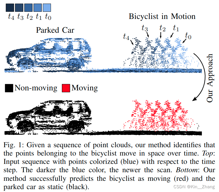
在自动驾驶导航中 dynamics obstacle 对于轨迹规划很重要,所以如何识别动态障碍物是一个比较重要的问题
问题场景
现有方法:
- 使用BEV角度的LiDAR Image进入2D Conv CNN进行提取 temporal info,通常这种 projection 2D表示 是从3D里聚类 比如 kNN
- 在建图过程中,根据聚类和tracking进行检测 运动点云
以上方法都是offline 需要时间内所有的LiDAR;其他方法也有对比两相邻帧点云的
本文方法主要focus on object that in a limited time horizon
Contribution
可以通过short sequence的LiDAR信息预测moving objects
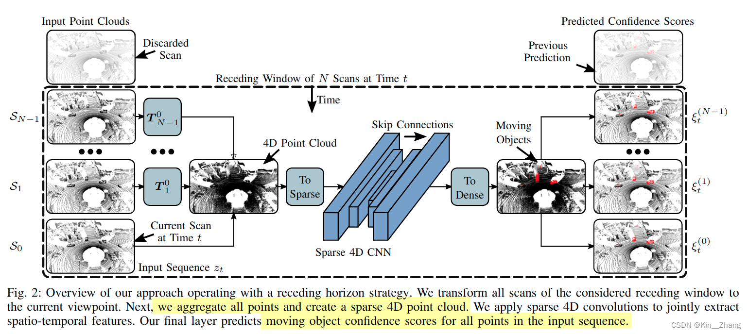
exploit sparse 4D Conv 从LiDAR点云中提取时空特征。方法输出:每个点云是否是动态物体的confidence scores,设计了一个一定大小的滑动窗口,超过一定删除旧frame
- 比现有方法 更精准的识别动态物体
- 对于unseen的场景有好的泛化性
- 通过在线新的观测输入,改进已知结果
2. Method
前提假设:已知所有帧帧之间的translation matrix \(\boldsymbol T\),point点表示 \(\boldsymbol{p}_{i}=\left[x_{i}, y_{i}, z_{i}, t_i\right]^{\top}\) ,因为室外的点云较为稀疏,所以将4D点云到sparse voxel grid,时间和空间的resolution分别为 \(\Delta t, \Delta s\)
使用一个稀疏的tensor保存voxel grid的indices和相关features
2.1 框架
2.2 Sparse 4D
稀疏4D卷积使用的是:Minkowski engine, NVIDIA做的一款开源的稀疏张量的自动微分库,比起dense conv,主要是为了加速
使用的是修改后的 MinkUNet14 [8],a sparse equivalent of a residual bottleneck architecture with strided sparse convolutions for downsampling the feature maps and strided sparse transpose convolutions for upsampling
不同于4D分割使用RGB作为input features,本文首先初始化voxels,被至少一个点占据时constant feature是0.5;因此我们的输入仅保存有点占据的voxel
这样部署到新环境下,不需要再考虑coordinates distribution或是通过intensity value对输入数据进行标准化了
下面为源码抽取的代码 进行的数据处理和sparse:
quantization = self.quantization.type_as(past_point_clouds[0])
past_point_clouds = [
   torch.div(point_cloud, quantization) for point_cloud in past_point_clouds
]
features = [
    0.5 * torch.ones(len(point_cloud), 1).type_as(point_cloud)
    for point_cloud in past_point_clouds
]

coords, features = ME.utils.sparse_collate(past_point_clouds, features)
tensor_field = ME.TensorField(
    features=features, coordinates=coords.type_as(features)
)

sparse_tensor = tensor_field.sparse()

predicted_sparse_tensor = self.MinkUNet(sparse_tensor)
2.3 Receding Horizon
经过上面的步骤后,网络会输出每个输入序列点上的confidence score。在实际运行网络时 inference time,避免重复输出同一帧的,一般是选择将输入数据进行切分固定;本文则是采取receding horizon,接收新的 就扔旧的 如上框架图
2.4 Binary Bayes Filter
本文的方法是直接预测的N个scan的输入,输出一个结果,receding horizon则可以通过接收新的一帧,re-estimate 前N-1的scans;对于多次预测结果我们使用binary bayes filter进行融合
贝叶斯融合层可以减少因为传感器噪音或被遮挡住时,输出错误的 false positive和negatives的数量

我们想预测的是 所有点在整个时间内对 motion state \(m^{(j)}\) 的联合概率:
\(m^{(j)} \in \{0,1\}\) 表示 点 \(p_i \in S_j\)的状态是否是moving,\(S_j\)为第j次扫描的LiDAR输入,后面的公式为了简洁点 把j就省去了哈
我们使用bayes’ rule在公式2上,然后follow standard derivation of the recursive binary bayes filter [36],下面的l为\(l(x)=\log \frac{p(x)}{1-p(x)}\) 通常在占用栅格地图上使用,如下进行更新:
prior probability \(p_0 \in (0,1)\) provides a measure of the innovation introduced by a new prediction. 这个值同样决定了how much 在单帧内的一个 predicted moving point 对于最后的prediction造成的影响
为网络输出的scores对应到上面moving的概率
则log-odds confidence的指数为:
然后经过公式3等,取回概率 \(p(x)=\log \frac{l(x)}{1+l(x)}\) 如果这个confidence score大于0.5 则认为这个点是移动的 反之是静止
代码对应
# Bayesian Fusion
elif strategy == "bayes":
    for pred_idx, confidences in tqdm(dict_confidences.items(), desc="Scans"):
        confidence = np.load(confidences[0])
        log_odds = prob_to_log_odds(confidence)
        for conf in confidences[1:]:
            confidence = np.load(conf)
            log_odds += prob_to_log_odds(confidence)
            log_odds -= prob_to_log_odds(prior * np.ones_like(confidence))
        final_confidence = log_odds_to_prob(log_odds)
        pred_labels = to_label(final_confidence, semantic_config)
        pred_labels.tofile(pred_path + "/" + pred_idx.split(".")[0] + ".label")
verify_predictions(seq, pred_path, semantic_config)

def to_label(confidence, semantic_config):
    pred_labels = np.ones_like(confidence)
    pred_labels[confidence > 0.5] = 2
    pred_labels = to_original_labels(pred_labels, semantic_config)
    pred_labels = pred_labels.reshape((-1)).astype(np.int32)
    return pred_labels
3. 实验及结果
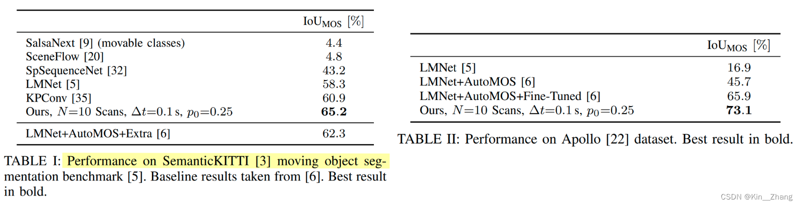
消融实验做的挺多,很仔细的,metric主要是针对运动物体所在的点的IoU
上面提到的\(p_0\)的赋值会产生IoU值的不同
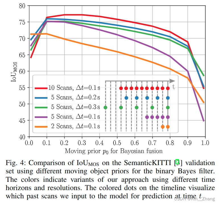

其中表三的\(\Delta t\) 为不同的时间分辨率下
对于运行的时间也有讨论,Python运行,整个网络如果是10次scans的话平均是0.078s,5次scans的话0.047s 在NVIDIA RTX A5000;bayes filter分别需要0.008s 0.004s对于10和5次
4. Conclusion
重复一下方法和contribution部分:
使用receding horizon对输入序列进行动态障碍物的预测,同时结合了binary bayes filter在时间维度上对预测结果进行融合,增加鲁棒性
未来工作可以在于里程计上的优化,因为在本文讨论时,里程计设置为已知状态。
赠人点赞 手有余香 😆;正向回馈 才能更好开放记录 hhh

 浙公网安备 33010602011771号