


对象测量
对象测量可以帮助我们进行矩阵计算:
- 获取弧长与面积
- 多边形拟合
- 计算图片对象中心
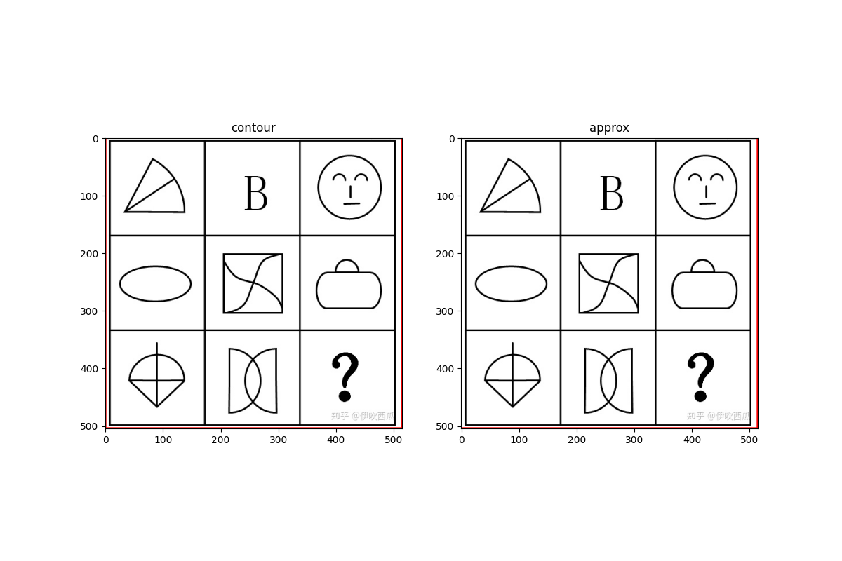
多边形拟合
步骤:
读取图片
转换成灰度图
二值化
轮廓检测
计算轮廓周长
多边形拟合
格式:
cv2.approxPolyDP(curve, epsilon, closed, approxCurve=None)
1
参数:
curve: 输入轮廓
epsilon: 逼近曲率, 越小表示相似逼近越厉害
closed: 是否闭合
import cv2
from matplotlib import pyplot as plt

# 读取图片
image = cv2.imread("tx.png")
image_gray = cv2.cvtColor(image, cv2.COLOR_BGR2GRAY)

# 二值化
ret, thresh = cv2.threshold(image_gray, 127, 255, cv2.THRESH_OTSU)

# 计算轮廓
contours, hierarchy = cv2.findContours(thresh, cv2.RETR_TREE, cv2.CHAIN_APPROX_NONE)

# 轮廓近似
perimeter = cv2.arcLength(contours[0], True)
approx = cv2.approxPolyDP(contours[0], perimeter * 0.1, True)

# 绘制轮廓
result1 = cv2.drawContours(image.copy(), contours, 0, (0, 0, 255), 2)
result2 = cv2.drawContours(image.copy(), [approx], -1, (0, 0, 255), 2)

# 图片展示
f, ax = plt.subplots(1, 2, figsize=(12, 8))

# 子图
ax[0].imshow(cv2.cvtColor(result1, cv2.COLOR_BGR2RGB))
ax[1].imshow(cv2.cvtColor(result2, cv2.COLOR_BGR2RGB))

# 标题
ax[0].set_title("contour")
ax[1].set_title("approx")

plt.show()
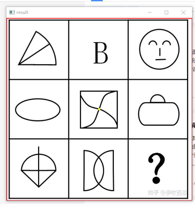
计算对象中心
cv2.moments()可以帮助我们得到轮距, 从而进一步计算图片对象的中心.
格式:
cv2.moments(array, binaryImage=None)
1
参数:
array: 轮廓
binaryImage: 是否把 array 内的非零值都处理为 1, 默认为 None
import numpy as np
import cv2

# 读取图片
image = cv2.imread("tx.png")
image_gray = cv2.cvtColor(image, cv2.COLOR_BGR2GRAY)

# 二值化
ret, thresh = cv2.threshold(image_gray, 0, 255, cv2.THRESH_OTSU)

# 获取轮廓
contours, hierarchy = cv2.findContours(thresh, cv2.RETR_EXTERNAL, cv2.CHAIN_APPROX_SIMPLE)

# 遍历每个轮廓
for i, contour in enumerate(contours):

    # 面积
    area = cv2.contourArea(contour)

    # 外接矩形
    x, y, w, h = cv2.boundingRect(contour)

    # 获取论距
    mm = cv2.moments(contour)
    print(mm, type(mm))  # 调试输出 (字典类型)

    # 获取中心
    cx = mm["m10"] / mm["m00"]
    cy = mm["m01"] / mm["m00"]

    # 获取
    cv2.circle(image, (np.int(cx), np.int(cy)), 3, (0, 255, 255), -1)
    cv2.rectangle(image, (x, y), (x + w, y + h), (0, 0, 255), 2)

# 图片展示
cv2.imshow("result", image)
cv2.waitKey(0)
cv2.destroyAllWindows()

# 保存图片
cv2.imwrite("result1.jpg", image)
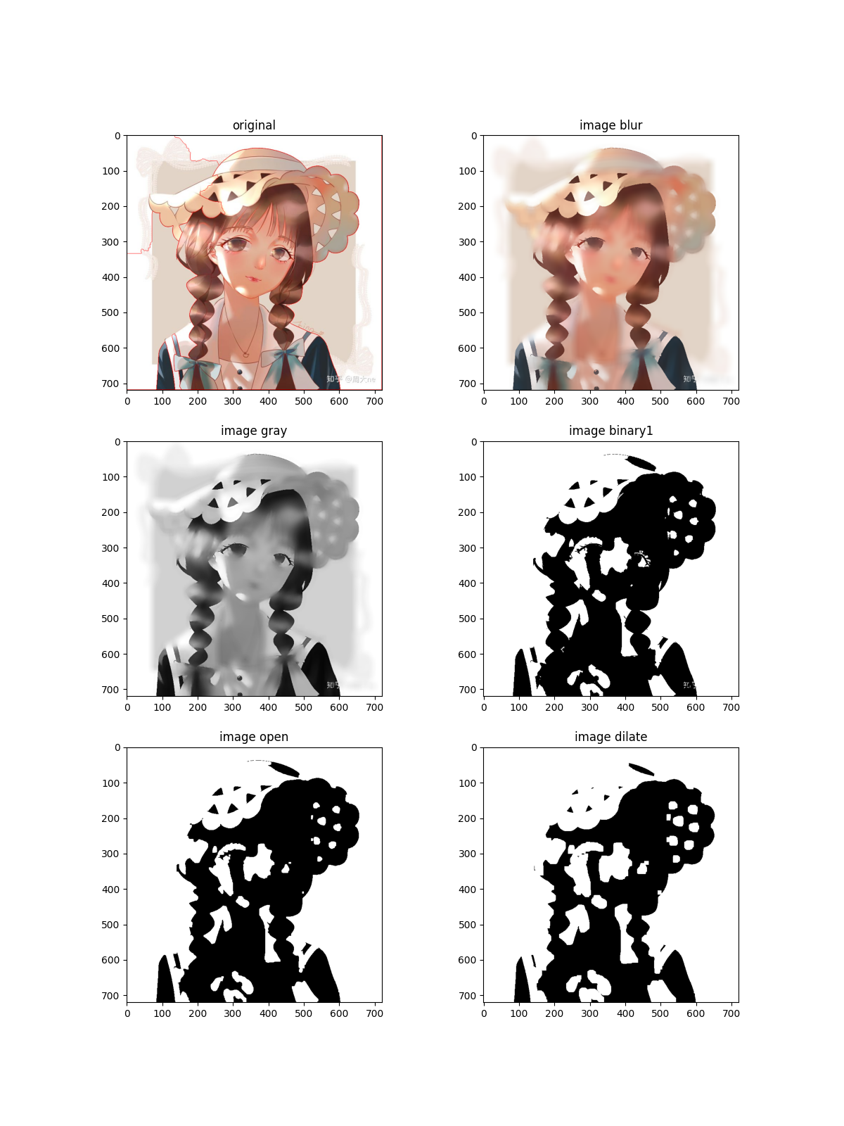
分水岭算法
分水岭算法 (Watershed Algorithm) 是一种图像区域分割算法. 在分割的过程中, 分水岭算法会把跟临近像素间的相似性作为重要的根据.
分水岭分割流程:
- 读取图片
- 转换成灰度图
- 二值化
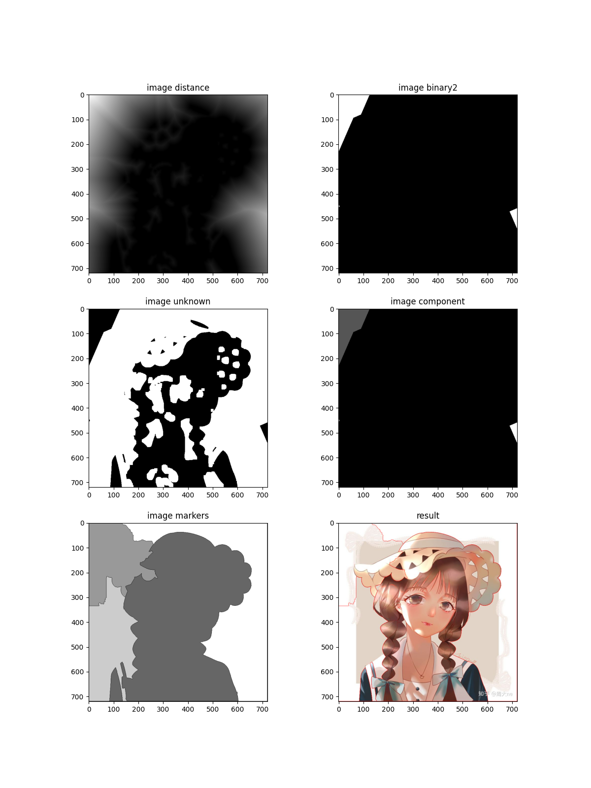
- 距离变换
- 寻找种子
- 生成 Marker
- 分水岭变换
连通域
连通域 (Connected Components) 指的是图像中具有相同像素且位置相邻的前景像素点组成的图像区域.
cv2.connectedComponents(image, labels=None, connectivity=None, ltype=None)
1
参数:
image: 输入图像, 必须是 uint8 二值图像
labels 图像上每一像素的标记, 用数字 1, 2, 3 表示
分水岭
算法会根据 markers 传入的轮廓作为种子, 对图像上其他的像素点根据分水岭算法规则进行判断, 并对每个像素点的区域归属进行划定. 区域之间的分界处的值被赋值为 -1.
cv2.watershed(image, markers)参数:
- image: 输入图像
- markers: 种子, 包含不同区域的轮廓
import numpy as np
import cv2
from matplotlib import pyplot as plt


def watershed(image):
    """分水岭算法"""

    # 卷积核
    kernel = cv2.getStructuringElement(cv2.MORPH_RECT, (3, 3))

    # 均值迁移滤波
    blur = cv2.pyrMeanShiftFiltering(image, 10, 100)

    # 转换成灰度图
    image_gray = cv2.cvtColor(blur, cv2.COLOR_BGR2GRAY)

    # 二值化
    ret1, thresh1 = cv2.threshold(image_gray, 0, 255, cv2.THRESH_OTSU)

    # 开运算
    open = cv2.morphologyEx(thresh1, cv2.MORPH_OPEN, kernel, iterations=2)

    # 膨胀
    dilate = cv2.dilate(open, kernel, iterations=3)

    # 距离变换
    dist = cv2.distanceTransform(dilate, cv2.DIST_L2, 3)
    dist = cv2.normalize(dist, 0, 1.0, cv2.NORM_MINMAX)
    print(dist.max())

    # 二值化
    ret2, thresh2 = cv2.threshold(dist, dist.max() * 0.6, 255, cv2.THRESH_BINARY)
    thresh2 = np.uint8(thresh2)

    # 分水岭计算
    unknown = cv2.subtract(dilate, thresh2)
    ret3, component = cv2.connectedComponents(thresh2)
    print(ret3)

    # 分水岭计算
    markers = component + 1
    markers[unknown == 255] = 0
    result = cv2.watershed(image, markers=markers)
    image[result == -1] = [0, 0, 255]

    # 图片展示
    image_show((image, blur, image_gray, thresh1, open, dilate), (dist, thresh2, unknown, component, markers, image))

    return image


def image_show(graph1, graph2):
    """绘制图片"""

    # 图像1
    original, blur, gray, binary1, open, dilate = graph1

    # 图像2
    dist, binary2, unknown, component, markers, result = graph2

    f, ax = plt.subplots(3, 2, figsize=(12, 16))

    # 绘制子图
    ax[0, 0].imshow(cv2.cvtColor(original, cv2.COLOR_BGR2RGB))
    ax[0, 1].imshow(cv2.cvtColor(blur, cv2.COLOR_BGR2RGB))
    ax[1, 0].imshow(gray, "gray")
    ax[1, 1].imshow(binary1, "gray")
    ax[2, 0].imshow(open, "gray")
    ax[2, 1].imshow(dilate, "gray")

    # 标题
    ax[0, 0].set_title("original")
    ax[0, 1].set_title("image blur")
    ax[1, 0].set_title("image gray")
    ax[1, 1].set_title("image binary1")
    ax[2, 0].set_title("image open")
    ax[2, 1].set_title("image dilate")

    plt.show()

    f, ax = plt.subplots(3, 2, figsize=(12, 16))

    # 绘制子图
    ax[0, 0].imshow(dist, "gray")
    ax[0, 1].imshow(binary2, "gray")
    ax[1, 0].imshow(unknown, "gray")
    ax[1, 1].imshow(component, "gray")
    ax[2, 0].imshow(markers, "gray")
    ax[2, 1].imshow(cv2.cvtColor(result, cv2.COLOR_BGR2RGB))

    # 标题
    ax[0, 0].set_title("image distance")
    ax[0, 1].set_title("image binary2")
    ax[1, 0].set_title("image unknown")
    ax[1, 1].set_title("image component")
    ax[2, 0].set_title("image markers")
    ax[2, 1].set_title("result")

    plt.show()


if __name__ == "__main__":
    # 读取图片
    image = cv2.imread("girl.png")

    # 分水岭算法
    result = watershed(image)

    # 保存结果
    cv2.imwrite("result.png", result)


 浙公网安备 33010602011771号